MATLAB Programming for
Numerical Analysis
Copyright © 2014 by César Pérez López
This work is subject to copyright. All rights are reserved by the Publisher, whether the whole or part of the material is concerned, specifically the rights of translation, reprinting, reuse of illustrations, recitation, broadcasting, reproduction on microfilms or in any other physical way, and transmission or information storage and retrieval, electronic adaptation, computer software, or by similar or dissimilar methodology now known or hereafter developed. Exempted from this legal reservation are brief excerpts in connection with reviews or scholarly analysis or material supplied specifically for the purpose of being entered and executed on a computer system, for exclusive use by the purchaser of the work. Duplication of this publication or parts thereof is permitted only under the provisions of the Copyright Law of the Publisher’s location, in its current version, and permission for use must always be obtained from Springer. Permissions for use may be obtained through RightsLink at the Copyright Clearance Center. Violations are liable to prosecution under the respective Copyright Law.
ISBN-13 (pbk): 978-1-4842-0296-8
ISBN-13 (electronic): 978-1-4842-0295-1
Trademarked names, logos, and images may appear in this book. Rather than use a trademark symbol with every occurrence of a trademarked name, logo, or image we use the names, logos, and images only in an editorial fashion and to the benefit of the trademark owner, with no intention of infringement of the trademark.
The use in this publication of trade names, trademarks, service marks, and similar terms, even if they are not identified as such, is not to be taken as an expression of opinion as to whether or not they are subject to proprietary rights.
While the advice and information in this book are believed to be true and accurate at the date of publication, neither the authors nor the editors nor the publisher can accept any legal responsibility for any errors or omissions that may be made. The publisher makes no warranty, express or implied, with respect to the material contained herein.
Publisher: Heinz Weinheimer Lead Editor: Dominic Shakeshaft
Editorial Board: Steve Anglin, Mark Beckner, Ewan Buckingham, Gary Cornell, Louise Corrigan, Jim DeWolf, Jonathan Gennick, Jonathan Hassell, Robert Hutchinson, Michelle Lowman, James Markham,
Matthew Moodie, Jeff Olson, Jeffrey Pepper, Douglas Pundick, Ben Renow-Clarke, Dominic Shakeshaft, Gwenan Spearing, Matt Wade, Steve Weiss
Coordinating Editor: Jill Balzano
Distributed to the book trade worldwide by Springer Science+Business Media New York, 233 Spring Street, 6th Floor, New York, NY 10013. Phone 1-800-SPRINGER, fax (201) 348-4505, e-mail [email protected], or visit www.springeronline.com Apress Media, LLC is a California LLC and the sole member (owner) is Springer Science + Business Media Finance Inc (SSBM Finance Inc). SSBM Finance Inc is a Delaware corporation.f
For information on translations, please e-mail [email protected], or visit www.apress.com.
Apress and friends of ED books may be purchased in bulk for academic, corporate, or promotional use. eBook versions and licenses are also available for most titles. For more information, reference our Special Bulk Sales–eBook Licensing web page at www.apress.com/bulk-sales.
Any source code or other supplementary material referenced by the author in this text is available to readers at www.apress.com. For detailed information about how to locate your book’s source code, go to
For your convenience Apress has placed some of the front
matter material after the index. Please use the Bookmarks
Contents at a Glance
About the Author ...
ix
Chapter 1: The MATLAB Environment
■
...1
Chapter 2: MATLAB Language: Variables, Numbers, Operators and Functions
■
...29
Chapter 3: M
■
ATLAB Language: Development Environment Features ...83
Chapter 4: MATLAB Language: M-Files, Scripts, Flow Control and
■
Numerical Analysis Functions ...
121
Chapter 5: Numerical Algorithms: Equations, Derivatives and Integrals
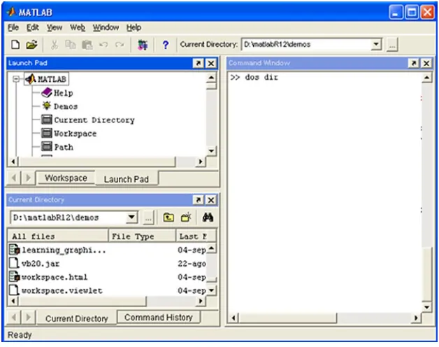
The MATLAB Environment
Starting MATLAB on Windows. The MATLAB working environment
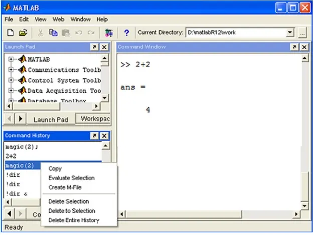
To start MATLAB, simply double-click on the shortcut icon to the program on the Windows desktop. Alternatively, if there is no desktop shortcut, the easiest and most common way to run the program is to choose programs from the Windows Start menu and select MATLAB. Having launched MATLAB by either of these methods, the welcome screen briefly appears, followed by the screen depicted in Figure 1-1, which provides the general environment in which the program works.
The most important elements of the MATLAB screen are the following:
• The Command Window: This runs MATLAB functions.
• The Command History: This presents a history of the functions introduced in the Command Window and allows you to copy and execute them.
• The Launch Pad: This runs tools and gives you access to documentation for all MathWorks products currently installed on your computer.
• The Current Directory: This shows MATLAB files and execute files (such as opening and search for content operations).
• Help (support): This allows you to search and read the documentation for the complete family of MATLAB products.
• The Workspace: This shows the present contents of the workspace and allows you to make changes to it.
• The Array Editor: This displays the contents of arrays in a tabular format and allows you to edit their values.
• The Editor/Debugger: This allows you to create, edit, and check M-files (files that contain MATLAB functions).
The MATLAB Command Window
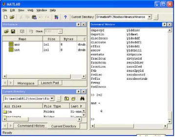
The Command Window (Figure 1-2) is the main way to communicate with MATLAB. It appears on the desktop when MATLAB starts and is used to execute all operations and functions. The entries are written to the right of the prompt >> and, once completed, they run after pressing Enter. The first line of Figure 1-3 defines a matrix and, after pressing Enter, the matrix itself is displayed as output.
In the Command Window, it is possible to evaluate previously executed operations. To do this, simply select the syntax you wish to evaluate, right-click, and choose the option Evaluate Selection from the resulting pop-up menu (Figures 1-4 and 1-5). Choosing Open Selection from the same menu opens in the Editor/Debugger an M-file previously selected in the Command Window (Figures 1-6 and 1-7).
Figure 1-3.
Figure 1-5.
MATLAB is sensitive to the use of uppercase and lowercase characters, and blank spaces can be used before and after minus signs, colons and parentheses. MATLAB also allows you to write several commands on the same line, provided they are separated by semicolons (Figure 1-8). Entries are executed sequentially in the order they appear on the line. Every command which ends with a semicolon will run, but will not display its output.
Long entries that will not fit on one line can be continued onto a second line by placing dots at the end of the first line (Figure 1-9).
Figure 1-9.
Figure 1-10.
The option Clear Command Window from the Edit menu (Figure 1-10) allows you to clear the Command Window. The command clc also performs this function (Figure 1-11). Similarly, the options Clear Command History
To help you to easily identify certain elements as if/else instructions, chains, etc., some entries in the Command Window will appear in different colors. Some of the existing rules for colors are as follows:
1. Chains appear in purple while they are being typed. When they are finished properly (with a closing quote) they become brown.
2. Flow control syntax appears in blue. All lines between the opening and closing of the flow control functions are correctly indented.
3. Parentheses, brackets, and keys are briefly illuminated until their contents are properly completed. This allows the user to easily see if mathematical expressions are properly closed.
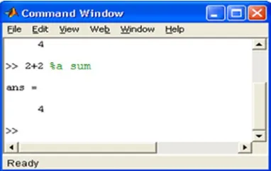
4. Comments in the Command Window, preceded by the symbol %, appear in green.
5. System commands such as ! appear in gold.
6. Errors are shown in red.
Below is a list of keys, arrows and combinations that can be used in the Command Window.
Key
Control key
Operation
� CTRL+ p Calls to the last entry submitted.
¯ CTRL+ n Calls to the next line.
← CTRL+ b Moves one character backward.
Key
Control key
Operation
End CTRL+ e Moves the end of the line. ESC CTRL+ u Deletes the line.
Delete CTRL+ d Deletes the character where the cursor is. BACKSPACE CTRL+ h Deletes the character before the cursor.
CTRL+ k Deletes all text up to the end of the line.
Shift+ home Highlights the text from the beginning of the line.
Shift+ end Highlights the text up to the end of the line.
Figure 1-13. Figure 1-12.
To enter explanatory comments simply start them with the symbol % anywhere in a line. The rest of the line should be used for the comment (see Figure 1-12).
Running M-files (files that contain MATLAB code) follows the same procedure as running any other command or function. Just type the name of the M-file (with its arguments, if necessary) in the Command Window, and press
Enter (Figure 1-13). To see each function of an M-file as it runs, first enter the command echo on. To interrupt the execution of an M-file use CTRL + c or CTRL + break.
Escape and exit to DOS environment commands
There are three ways to pass from the MATLAB Command Window to the MS-DOS operating system environment to run temporary assignments.
Entering the command ! dos_command in the Command Window allows you to execute the specified command
dos_command in the MATLAB environment. Figure 1-14 shows the execution of the command ! dir. The same effect is achieved with the command dos dos_command (Figure 1-15).
Figure 1-14.
Figure 1-15.
Not only DOS commands, but also all kinds of executable files or batch tasks can be executed with the three previous commands. To leave MATLAB simply type quit or exit in the Command Window and then press Enter. Alternatively you can select the option Exit MATLAB from the File menu (Figure 1-17).
Figure 1-16.
Figure 1-17.
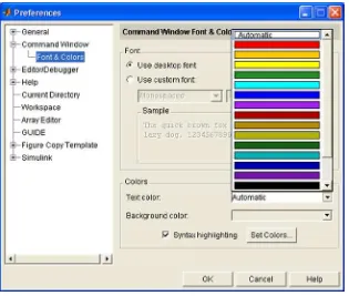
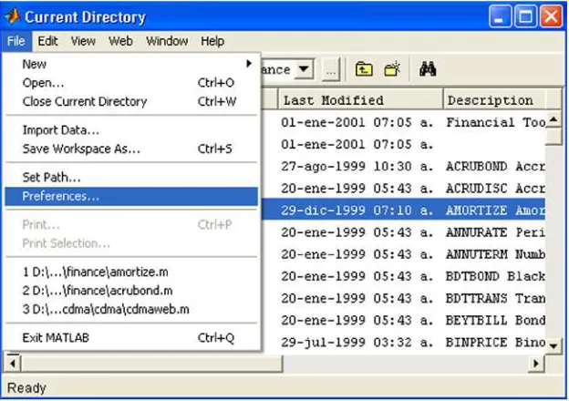
Preferences for the Command Window
Selecting the Preferences option from the File menu (Figure 1-18) allows you to set particular features for working in the Command Window. To do this, simply choose the desired options in the Command Window Preferences
Figure 1-18.
The first area that appears in the Command Window Preferences window is Text display. This specifies how the output will appear in the Command Window. Your options are as follows:
• Numeric format: Specifies the format of numerical values in the Command Window (Figure 1-21). This affects only the appearance of the numbers, not the calculations or how to save them. The possible formats are presented in the following table:
Format
Result
Example
+ +,-, white +
Bank Fixed 3.14
Compact Removes excess lines displayed on the screen to present a more compact output.
theta = pi/2 theta = 1.5708
Hex Hexadecimal 400921fb54442d18
long 15 digits fixed point 3.14159265358979
long e 15 digits floating-point 3. 141592653589793e + 00 long g The best of the previous two 3.14159265358979 loose Adds lines to make the output more readable.
The compact command does the opposite.
theta = pi/2 theta=1.5708
rat Ratio of small integers 355/13 (a rational approximation of pi)
short 5 digits fixed point 3.1416
short e 5 digits floating-point 3. 1416e + 00 short g The best of the previous two 3.1416
• Numeric display: Regulates the spacing of the output in the Command Window. Compact is used to suppress blank lines. Loose is used to show blank lines.
• Spaces per tab: Regulates the number of spaces assigned to the tab when the output is displayed (the default value is 4).
The second zone that appears in the Command Window Preferences window is Display. This specifies the size of the buffer and allows you to choose whether to display the executions of all the commands included in M-files. Your options are as follows:
• Echo on: If you check this box, the executions of all the commands included in the M-files are displayed.
• Limit matrix display width to eighty columns: If you check this box, MATLAB will display only an 80-column dot matrix output, regardless of the width of the Command Window. If this box is not checked, the matrix output will occupy the current width of the Command Window.
• Enable up to n tab completions: Check this box if you want to use tab completion when typing functions in the Command Window. You then need to specify the maximum number of completions that will be listed. If the number of possible completions exceeds this number, MATLAB will not show the list of completions.
• Command session scroll buffer size: This sets the number of lines that are kept in the Command Window buffer. These lines can be viewed by scrolling up.
In MATLAB it is also possible to set fonts and colors for the Command Window. To do this, simply unfold the sub-option Font & Colors hanging from Command Windows (Figure 1-21). In the fonts area select Use desktop font
To display the MATLAB Command Window separately simply click on the button located in the top right corner. To return the window to its site on the desktop, use the option Dock Command Window from the View menu (Figure 1-25).
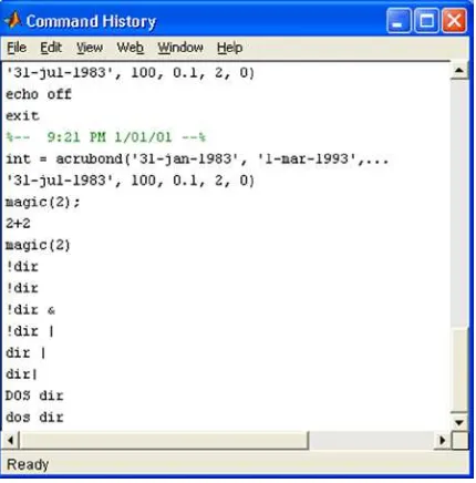
The Command History window
The Command History window (Figure 1-26) appears when you start MATLAB. It is located at the bottom right of the MATLAB desktop. The Command History window shows a list of functions used recently in the Command Window (Figure 1-26). It also shows an indicator of the beginning of the session. To display this window, separated from the MATLAB desktop, simply click on the button located in its top right corner. To return the window to its site on the desktop, use the Dock Window Command from the View menu. This method of separation and docking is common to all MATLAB windows.
Figure 1-26.
The Launch Pad window
The Launch Pad window (located by default in the upper-left corner of the MATLAB desktop) allows you to get help, see demonstrations of installed products, go to other windows on the desktop and visit the MathWorks website (Figure 1-28).
Figure 1-29.
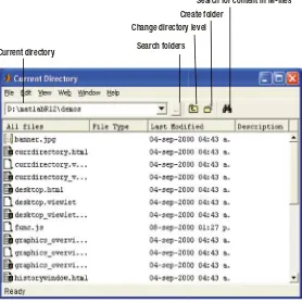
The Current Directory window
It is possible to set preferences in the Current Directory window using the Preferences option from the File menu (Figure 1-31). This gives you the Current Directory Preferences window (Figure 1-32). In the History field the number of recent directories is set to save to history. In the field Browser display options file characteristics are set to display (file type, date of last modification, and descriptions and comments from the M-files).
Search for content in M-files
Create folder
Change directory level
Current directory Search folders
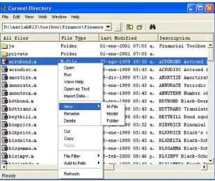
If you select any file in the Current Directory window and you left-click on it, the pop-up menu of Figure 1-33 will appear. This gives you options to open the file (Open), run it (Run), view Help (View Help), open it as text (Open as Text), import data (Import Data), create new files, M-files or folders (New), rename it, delete it, cut it, copy it or paste it, pass you filters and add it to the current path.
Figure 1-33.
The help browser
MATLAB’s help browser is obtained by clicking the button on the toolbar or by using the function helpbrowser in the Command Window.
The Workspace window
Figure 1-34.
Variable name
Read workspace variable type Save workspace size in bytes
An important element of the Workspace window is the Array editor, which allows you to edit numeric arrays and strings.
It is possible to set preferences in the Workspace window via the Preferences option from the File menu. This gives you the Preferences window shown in Figure 1-36. In the History field the number of recent directories is set to save to history. In the Font field the sources to be used in the Command Window preferences are set, and the option Confirm Deletion of Variables is checked according to whether or not you want the deletion of variables to be confirmed.
Figure 1-36.
The Editor and Debugger for M-files
To create a new M-file in the Editor/Debugger simply click the button in the MATLAB Tools toolbar or select
You can also open the Editor/Debugger by right-clicking anywhere in the Current Directory window and choosing
New ➤ M-file from the resulting pop-up menu (Figure 1-39). The option Open is used to open an existing M-file. You can open several M-files simultaneously, in which case they will appear in different windows (Figure 1-40).
Figure 1-40.
Help in MATLAB
Figure 1-41.
Another very important way to obtain help in MATLAB is via its support functions. These functions are presented in the following table.
Function
Description
doc function Displays the reference page in the browser’s support for the specified function, showing syntax, description, examples and links with other related functions.
docopt This function is used to display the location of the help files on UNIX platforms that do not support Java interfaces.
help function Displays in the Command Window a description and the syntax of the specified function.
helpbrowser Opens the help browser.
helpdesk Opens the help browser. It has been replaced by doc in recent versions of MATLAB.
helpwin or helpwin theme Displays in the help browser a list of all the MATLAB functions or those relating to the specified topic.
lookfor text Displays in the browser all support functions which contain the specified text as part of the function.
MATLAB Language: Variables,
Numbers, Operators and
Functions
Variables
MATLAB does not require a command to declare variables. A variable is created simply by directly allocating a value to it. For example:
>> v = 3
v =
3
The variable v will take the value 3 and using a new mapping will not change its value. Once the variable is declared, we can use it in calculations.
>> v ^ 3
ans =
27
>> v+5
ans =
8
If we now write:
>> v = 3 + 7
v =
10
then the variable v has the value 10 from now on, as shown in the following calculation:
>> v ^ 4
ans =
10000
A variable name must begin with a letter followed by any number of letters, digits or underscores. However, bear in mind that MATLAB uses only the first 31 characters of the name of the variable. It is also very important to note that MATLAB is case sensitive. Therefore, a variable named with uppercase letters is different to the variable with the same name except in lowercase letters.
Vector variables
A vector variable of n elements can be defined in MATLAB in the following ways:
V = [v1, v2, v3,..., vn]
V = [v1 v2 v3... vn]
When most MATLAB commands and functions are applied to a vector variable the result is understood to be that obtained by applying the command or function to each element of the vector:
>> vector1 = [1,4,9,2.25,1/4]
vector1 =
1.0000 4.0000 9.0000 2.2500 0.2500
>> sqrt (vector1)
ans =
1.0000 2.0000 3.0000 1.5000 0.5000
variable = [a:b] Defines the vector whose first and last elements are a and b, respectively, and the intermediate elements differ by one unit. variable = [a:s:b] Defines the vector whose first and last elements are a and b,
respectively, and the intermediate elements differ by an increase specified by s.
variable = linespace [a, b, n] Defines the vector with n evenly spaced elements whose first and last elements are a and b respectively.
variable = logspace [a, b, n] Defines the vector with n evenly logarithmically spaced elements whose first and last elements are 10aand 10b, respectively.
Below are some examples:
>> vector2 = [5:5:25]
vector2 =
5 10 15 20 25
This yields the numbers between 5 and 25, inclusive, separated by 5 units.
>> vector3=[10:30]
vector3 =
Columns 1 through 13
10 11 12 13 14 15 16 17 18 19 20 21 22
Columns 14 through 21
23 24 25 26 27 28 29 30
This yields the numbers between 10 and 30, inclusive, separated by a unit.
>> t:Microsoft.WindowsMobile.DirectX.Vector4 = linspace (10,30,6)
t:Microsoft.WindowsMobile.DirectX.Vector4 =
10 14 18 22 26 30
This yields 6 equally spaced numbers between 10 and 30, inclusive.
>> vector5 = logspace (10,30,6)
vector5 =
This yields 6 evenly logarithmically spaced numbers between 1010 and 1030, inclusive.
One can also consider row vectors and column vectors in MATLAB. A column vector is obtained by separating its elements by semicolons, or by transposing a row vector using a single quotation mark at the end of its definition.
>> a=[10;20;30;40]
You can also select an element of a vector or a subset of elements. The rules are summarized in the following table:
x (n) Returns the n-th element of the vector x.
x(a:b) Returns the elements of the vector x between the a-th and the b-th elements, inclusive.
x(a:p:b) Returns the elements of the vector x located between the a-th and the b-th elements, inclusive, but separated by p units (a > b).
x(b:-p:a) Returns the elements of the vector x located between the b-th and a-th elements, both inclusive, but separated by p units and starting with the b-th element (b > a).
This yields the sixth element of the vector x.
>> x(4:7)
ans =
4 5 6 7
This yields the elements of the vector x located between the fourth and seventh elements, inclusive.
>> x(2:3:9)
ans =
2 5 8
This yields the three elements of the vector x located between the second and ninth elements, inclusive, but separated in steps of three units.
>> x(9:-3:2)
ans =
9 6 3
This yields the three elements of the vector x located between the ninth and second elements, inclusive, but separated in steps of three units and starting at the ninth.
Matrix variables
MATLAB defines arrays by inserting in brackets all its row vectors separated by a comma. Vectors can be entered by separating their components by spaces or by commas, as we already know. For example, a 3 × 3 matrix variable can be entered in the following two ways:
M = [a11 a12 a13;a21 a22 a23;a31 a32 a33]
M = [a11,a12,a13;a21,a22,a23;a31,a32,a33]
A(m,n) Defines the (m, n)-th element of the matrix A (row m and column n).
A(a:b,c:d) Defines the subarray of A formed between the a-th and the b-th rows and between the c-th and the d-th columns, inclusive.
A(a:p:b,c:q:d) Defines the subarray of A formed by every p-th row between the a-th and the b-th rows, inclusive, and every q-th column between the c-th and the d-th column, inclusive.
A([a b],[c d]) Defines the subarray of A formed by the intersection of the a-th through b-th rows and c-th through d-th columns, inclusive.
A([a b c...], [e f g...])
Defines the subarray of A formed by the intersection of rows a, b, c,... and columns e, f, g,...
A(:,c:d) Defines the subarray of A formed by all the rows in A and the c-th through to the d-th columns. A(:,[c d e...]) Defines the subarray of A formed by all the rows in A and columns c, d, e,...
A(a:b,:) Defines the subarray of A formed by all the columns in A and the a-th through to the b-th rows. A([a b c...],:) Defines the subarray of A formed by all the columns in A and rows a, b, c,...
A(a,:) Defines the a-th row of the matrix A. A(:,b) Defines the b-th column of the matrix A.
A(:) Defines a column vector whose elements are the columns of A placed in order below each other. A(:,:) This is equivalent to the entire matrix A.
[A, B, C,...] Defines the matrix formed by the matrices A, B, C,...
SA= [ ] Clears the subarray of the matrix A, SA, and returns the remainder. diag (v) Creates a diagonal matrix with the vector v in the diagonal. diag (A) Extracts the diagonal of the matrix as a column vector. eye (n) Creates the identity matrix of order n.
eye (m, n) Create an m×n matrix with ones on the main diagonal and zeros elsewhere. zeros (m, n) Creates the zero matrix of order m×n.
ones (m, n) Creates the matrix of order m×n with all its elements equal to 1. rand (m, n) Creates a uniform random matrix of order m×n.
randn (m, n) Create a normal random matrix of order m×n.
flipud (A) Returns the matrix whose rows are those of A but placed in reverse order (from top to bottom). fliplr (A) Returns the matrix whose columns are those of A but placed in reverse order (from left to right). rot90 (A) Rotates the matrix A counterclockwise by 90 degrees.
reshape(A, m, n) Returns an m×n matrix formed by taking consecutive entries of A by columns. size (A) Returns the order (size) of the matrix A.
find (condA) Returns all A items that meet a given condition. length (v) Returns the length of the vector v.
tril (A) Returns the lower triangular part of the matrix A. triu (A) Returns the upper triangular part of the matrix A. A' Returns the transpose of the matrix A.
Here are some examples:
We consider first the 2 × 3 matrix whose rows are the first six consecutive odd numbers:
>> A = [1 3 5; 7 9 11]
We now construct a matrix C, formed by attaching the identity matrix of order 3 to the right of the matrix B:
>> C = [B eye (3)] intersection of the first two rows of C and its third and fifth columns, and a matrix F formed by taking the intersection of the first two rows and the last three columns of the matrix C:
>> D = C(:,1:2:5)
D =
>> E = C([1 2],[3 5])
Now we build the diagonal matrix G such that the elements of the main diagonal are the same as those of the main diagonal of D:
We then build the matrix H, formed by taking the intersection of the first and third rows of C and its second, third and fifth columns:
>> H = C([1 3],[2 3 5])
H =
7 1 0 0 0 1
Now we build an array I formed by the identity matrix of order 5 × 4, appending the zero matrix of the same order to its right and to the right of that the unit matrix, again of the same order. Then we extract the first row of I and, finally, form the matrix J comprising the odd rows and even columns of I and calculate its order (size).
>> I = [eye(5,4) zeros(5,4) ones(5,4)]
>> I(1,:) columns of K and then perform both operations simultaneously. Finally, we find the matrix L of order 4 × 3 whose columns are obtained by taking the elements of K sequentially by columns.
>> K(3:-1:1,4:-1:1)
A character variable (chain) is simply a character string enclosed in single quotes that MATLAB treats as a vector form. The general syntax for character variables is as follows:
c = 'string'
Among the MATLAB commands that handle character variables we have the following:
abs ('character_string') Returns the array of ASCII characters equivalent to each character in the string. setstr (numeric_vector) Returns the string of ASCII characters that are equivalent to the elements of the vector. str2mat (t1,t2,t3,...) Returns the matrix whose rows are the strings t1, t2, t3,..., respectively.
str2num ('string') Converts the string to its exact numeric value used by MATLAB. num2str (number) Returns the exact number in its equivalent string with fixed precision. int2str (integer) Converts the integer to a string.
sprintf ('format', a) Converts a numeric array into a string in the specified format. sscanf ('string', 'format') Converts a string to a numeric value in the specified format. dec2hex (integer) Converts a decimal integer into its equivalent string in hexadecimal. hex2dec ('string_hex') Converts a hexadecimal string into its integer equivalent.
hex2num ('string_hex') Converts a hexadecimal string into the equivalent IEEE floating point number. lower ('string') Converts a string to lowercase.
upper ('string') Converts a string to uppercase.
strcmp (s1, s2) Compares the strings s1 and s2 and returns 1 if they are equal and 0 otherwise. strcmp (s1, s2, n) Compares the strings s1 and s2 and returns 1 if their first n characters are equal
and 0 otherwise.
strrep (c, 'exp1', 'exp2') Replaces exp1 by exp2 in the chain c. findstr (c, 'exp') Finds where exp is in the chain c.
isstr (expression) Returns 1 if the expression is a string and 0 otherwise.
ischar (expression) Returns 1 if the expression is a string and 0 otherwise. strjust (string) Right justifies the string.
blanks (n) Generates a string of n spaces.
deblank (string) Removes blank spaces from the right of the string. eval (expression) Executes the expression, even if it is a string.
disp (‘string’) Displays the string (or array) as has been written, and continues the MATLAB process. input (‘string’) Displays the string on the screen and waits for a key press to continue.
Here are some examples:
>> hex2dec ('3ffe56e')
ans =
67102062
Here MATLAB has converted a hexadecimal string into a decimal number.
>> dec2hex (1345679001)
ans =
50356E99
The program has converted a decimal number into a hexadecimal string.
>> sprintf(' %f',[1+sqrt(5)/2,pi])
ans =
2.118034 3.141593
The exact numerical components of a vector have been converted to strings (with default precision).
>> sscanf('121.00012', '%f')
ans =
121.0001
Here a numeric string has been passed to an exact numerical format (with default precision).
>> num2str (pi)
ans =
The constant p has been converted into a string.
>> str2num('15/14')
ans =
1.0714
The string has been converted into a numeric value with default precision.
>> setstr(32:126)
ans =
!"#$% &' () * +, -. / 0123456789:; < = >? @ABCDEFGHIJKLMNOPQRSTUVWXYZ [\] ^ _'abcdefghijklmnopqrstuvwxyz {|}~
This yields the ASCII characters associated with the whole numbers between 32 and 126, inclusive.
>> abs('{]}><#¡¿?ºª')
ans =
123 93 125 62 60 35 161 191 63 186 170
This yields the integers corresponding to the ASCII characters specified in the argument of abs.
>> lower ('ABCDefgHIJ')
ans =
abcdefghij
The text has been converted to lowercase.
>> upper('abcd eFGHi jKlMn')
ans =
ABCD EFGHI JKLMN
The text has been converted to uppercase.
>> str2mat ('The world',' The country',' Daily 16', ' ABC')
ans =
The chains comprising the arguments of str2mat have been converted to a text array.
>> disp('This text will appear on the screen')
ans =
This text will appear on the screen
Here the argument of the command disp has been displayed on the screen.
>> c = 'This is a good example'; >> strrep(c, 'good', 'bad')
ans =
This is a bad example
The string good has been replaced by bad in the chain c. The following instruction locates the initial position of each occurrence of is within the chain c.
>> findstr (c, 'is')
ans =
3 6
Numbers
In MATLAB the arguments of a function can take many different forms, including different types of numbers and numerical expressions, such as integers and rational, real and complex numbers.
Arithmetic operations in MATLAB are defined according to the standard mathematical conventions. MATLAB is an interactive program that allows you to perform a simple variety of mathematical operations. MATLAB assumes the usual operations of sum, difference, product, division and power, with the usual hierarchy between them:
x + y Sum
x – y Difference x * y or x y Product
x/y Division
To add two numbers simply enter the first number, a plus sign (+) and the second number. Spaces may be included before and after the sign to ensure that the input is easier to read.
>> 2 + 3
ans =
5
We can perform power calculations directly.
>> 100 ^ 50
ans =
1. 0000e + 100
Unlike a calculator, when working with integers, MATLAB displays the full result even when there are more digits than would normally fit across the screen. For example, MATLAB returns the following value of 99 ^ 50 when using the vpa function (here to the default accuracy of 32 significant figures).
>> vpa '99 ^ 50'
ans =
. 60500606713753665044791996801256e100
To combine several operations in the same instruction one must take into account the usual priority criteria among them, which determine the order of evaluation of the expression. Consider, for example:
>> 2 * 3 ^ 2 + (5-2) * 3
ans =
27
Taking into account the priority of operators, the first expression to be evaluated is the power 3^2. The usual evaluation order can be altered by grouping expressions together in parentheses.
In addition to these arithmetic operators, MATLAB is equipped with a set of basic functions and you can also define your own functions. MATLAB functions and operators can be applied to symbolic constants or numbers.
One of the basic applications of MATLAB is its use in realizing arithmetic operations as if it were a conventional calculator, but with one important difference: the precision of the calculation. Operations are performed to whatever degree of precision the user desires. This unlimited precision in calculation is a feature which sets MATLAB apart from other numerical calculation programs, where the accuracy is determined by a word length inherent to the software, and cannot be modified.
format long Delivers results to 16 significant decimal figures.
format short Delivers results to 4 decimal places. This is MATLAB’s default format. format long e Provides the results to 16 decimal figures more than the power of 10 required. format short e Provides the results to four decimal figures more than the power of 10 required. format long g Provides the results in optimal long format.
format short g Provides the results in optimum short format. bank format Delivers results to 2 decimal places.
format rat Returns the results in the form of a rational number approximation. format + Returns the sign (+, -) and ignores the imaginary part of complex numbers. format hex Returns results in hexadecimal format.
vpa ‘operations’ n Returns the result of the specified operations to n significant digits.
numeric (‘expr’) Provides the value of the expression numerically approximated by the current active format. digits (n) Returns results to n significant digits.
Using format gives a numerical approximation of 174/13 in the way specified after the format command:
>> 174/13
>> format long e; 174/13
ans =
1.338461538461539e + 001
>> format short e; 174/13
ans =
1.3385e + 001
>> format long g; 174/13
ans =
>> format short g; 174/13
Now we will see how the value of sqrt (17) can be calculated to any precision that we desire:
>> vpa ' 174/13 ' 10
In MATLAB all common operations with whole numbers are exact, regardless of the size of the output. If we want the result of an operation to appear on screen to a certain number of significant figures, we use the symbolic computation command vpa (variable precision arithmetic), whose syntax we already know.
For example, the following calculates 6^400 to 450 significant figures:
The result of the operation is precise, always displaying a point at the end of the result. In this case it turns out that the answer has fewer than 450 digits anyway, so the solution is exact. If you require a smaller number of significant figures, that number can be specified and the result will be rounded accordingly. For example, calculating the above power to only 50 significant figures we have:
>> '6 vpa ^ 400' 50
ans =
. 18217977168218728251394687124089371267338971528175e312
Functions of integers and divisibility
There are several functions in MATLAB with integer arguments, the majority of which are related to divisibility. Among the most typical functions with integer arguments are the following:
rem (n, m) Returns the remainder of the division of n by m (also valid when n and m are real).
sign (n) The sign of n (i.e. 1 if n > 0, - 1 if n < 0). max (n1, n2) The maximum of n1 and n2.
min (n1, n2) The minimum of n1 and n2.
gcd (n1, n2) The greatest common divisor of n1 and n2. lcm (n1, n2) The least common multiple of n1 and n2. factorial (n) n factorial (i.e. n(n-1) (n-2)...1)
factor (n) Returns the prime factorization of n.
Below are some examples.
The remainder of division of 17 by 3:
>> rem (17,3)
ans =
2
The remainder of division of 4.1 by 1.2:
>> rem (4.1,1.2)
ans =
The remainder of division of -4.1 by 1.2:
>> rem(-4.1,1.2)
ans =
-0.5000
The greatest common divisor of 1000, 500 and 625:
>> gcd (1000, gcd (500,625))
ans =
125.00
The least common multiple of 1000, 500 and 625:
>> lcm (1000, lcm (500,625))
ans =
5000.00
Alternative bases
MATLAB allows you to work with numbers to any base, as long as the extended symbolic math Toolbox is available. It also allows you to express all kinds of numbers in different bases. This is implemented via the following functions:
dec2base (decimal, n_base) Converts the specified decimal number to the new base n_base. base2dec(number,b) Converts the given number in base b to a decimal number. dec2bin (decimal) Converts the specified decimal number to base 2 (binary). dec2hex (decimal) Converts the specified decimal number to base 16 (hexadecimal). bin2dec (binary) Converts the specified binary number to decimal.
hex2dec (hexadecimal) Converts the specified base 16 number to decimal.
Below are some examples.
Represent in base 10 the base 2 number 100101.
>> base2dec('100101',2)
ans =
Represent in base 10 the hexadecimal number FFFFAA00.
>> base2dec ('FFFFAA0', 16)
ans =
268434080.00
Represent the result of the base 16 operation FFFAA2+FF-1 in base 10.
>> base2dec('FFFAA2',16) + base2dec('FF',16)-1
ans =
16776096.00
Real numbers
As is well known, the set of real numbers is the disjoint union of the set of rational numbers and the set of irrational numbers. A rational number is a number of the form p/q, where p and q are integers. In other words, the rational numbers are those numbers that can be represented as a quotient of two integers. The way in which MATLAB treats rational numbers differs from the majority of calculators. If we ask a calculator to calculate the sum 1/2 + 1/3 + 1/4, most will return something like 1.0833, which is no more than an approximation of the result.
The rational numbers are ratios of integers, and MATLAB can work with them in exact mode, so the result of an arithmetic expression involving rational numbers is always given precisely as a ratio of two integers. To enable this, activate the rational format with the command format rat. If the reader so wishes, MATLAB can also return the results in decimal form by activating any other type of format instead (e.g. format short or format long). MATLAB evaluates the above mentioned sum in exact mode as follows:
>> format rat >> 1/2 + 1/3 + 1/4
ans =
13/12
Unlike calculators, MATLAB ensures its operations with rational numbers are accurate by maintaining the rational numbers in the form of ratios of integers. In this way, calculations with fractions are not affected by rounding errors, which can become very serious, as evidenced by the theory of errors. Note that, once the rational format is enabled, when MATLAB adds two rational numbers the result is returned in symbolic form as a ratio of integers, and operations with rational numbers will continue to be exact until an alternative format is invoked.
A floating point number, or a number with a decimal point, is interpreted as exact if the rational format is enabled. Thus a floating point expression will be interpreted as an exact rational expression while any irrational numbers in a rational expression will be represented by an appropriate rational approximation.
>> format rat >> 10/23 + 2.45/44
ans =
The other fundamental subset of the real numbers is the set of irrational numbers, which have always created difficulties in numerical calculation due to their special nature. The impossibility of representing an irrational number accurately in numeric mode (using the ten digits from the decimal numbering system) is the cause of most of the problems. MATLAB represents the results with an accuracy which can be set as required by the user. An irrational number, by definition, cannot be represented exactly as the ratio of two integers. If ordered to calculate the square root of 17, by default MATLAB returns the number 5.1962.
>> sqrt (27)
ans =
5.1962
MATLAB incorporates the following common irrational constants and notions:
pi The number p = 3.1415926... exp (1) The number e = 2.7182818...
Inf Infinity (returned, for example, when it encounters 1/0). NaN Uncertainty (returned, for example, when it encounters 0/0).
realmin Returns the smallest possible normalized floating-point number in IEEE double precision. realmax Returns the largest possible finite floating-point number in IEEE double precision.
The following examples illustrate how MATLAB outputs these numbers and notions.
>> realmin
ans =
2. 225073858507201e-308
>> realmax
ans =
1. 797693134862316e + 308
Functions with real arguments
The disjoint union of the set of rational numbers and the set of irrational numbers is the set of real numbers. In turn, the set of rational numbers has the set of integers as a subset. All functions applicable to real numbers are also valid for integers and rational numbers. MATLAB provides a full range of predefined functions, most of which are discussed in the subsequent chapters of this book. Within the group of functions with real arguments offered by MATLAB, the following are the most important:
Trigonometric functions
Function
Inverse
sin (x) asin (x)
cos (x) acos (x)
tan(x) atan(x) and atan2(y,x)
csc (x) acsc (x)
sec (x) asec (x)
cot (x) acot (x)
Hyperbolic functions
Function
Inverse
sinh (x) asinh (x)
cosh(x) acosh(x)
tanh(x) atanh(x)
csch(x) acsch(x)
sech(x) asech(x)
Exponential and logarithmic functions
Function
Meaning
exp (x) Exponential function in base e (e ^ x). log (x) Base e logarithm of x.
log10 (x) Base 10 logarithm of x. log2 (x) Base 2 logarithm of x. pow2 (x) 2 raised to the power x. sqrt (x) The square root of x.
Numeric variable-specific functions
Function
Meaning
abs (x) The absolute value of x.
floor (x) The largest integer less than or equal to x. ceil (x) The smaller integer greater than or equal to x. round (x) The closest integer to x.
fix (x) Removes the fractional part of x.
rem (a, b) Returns the remainder of the division of a by b. sign (x) Returns the sign of x (1 if x > 0,0 if x=0,- 1 if x < 0).
Here are some examples:
>> sin(pi/2)
ans =
1
>> asin (1)
ans =
1.57079632679490
>> log (exp (1) ^ 3)
ans =
The function round is demonstrated in the following two examples:
>> round (2.574)
ans =
3
>> round (2.4)
ans =
2
The function ceil is demonstrated in the following two examples:
>> ceil (4.2)
ans =
5
>> ceil (4.8)
ans =
5
The function floor is demonstrated in the following two examples:
>> floor (4.2)
ans =
4
>> floor (4.8)
ans =
4
The fix function simply removes the fractional part of a real number:
>> fix (5.789)
ans =
Complex numbers
Operations on complex numbers are well implemented in MATLAB. MATLAB follows the convention that i or j
represents the key value in complex analysis, the imaginary number √- 1. All the usual arithmetic operators can be applied to complex numbers, and there are also some specific functions which have complex arguments. Both the real and the imaginary part of a complex number can be a real number or a symbolic constant, and operations with them are always performed in exact mode, unless otherwise instructed or necessary, in which case an approximation of the result is returned. As the imaginary unit is represented by the symbol i or j, the complex numbers are expressed in the form a+bi or a+bj. Note that you don't need to use the product symbol (asterisk) before the imaginary unit:
>> (1-5i)*(1-i)/(-1+2i)
ans =
-1.6000 + 2.8000i
>> format rat
>> (1-5i) *(1-i) /(-1+2i)
ans =
-8/5 + 14/5i
Functions with complex arguments
Working with complex variables is very important in mathematical analysis and its many applications in engineering. MATLAB implements not only the usual arithmetic operations with complex numbers, but also various complex functions. The most important functions are listed below.
Trigonometric functions
Function
Inverse
sin (z) asin (z)
cos (z) acos (z)
tan (z) atan(z) and atan2(imag(z),real(z))
csc (z) acsc (z)
sec (z) asec (z)
Hyperbolic functions
exp (z) Exponential function in base e (e ^ z) log (z) Base e logarithm of z.
log10 (z) Base 10 logarithm of z. log2 (z) Base 2 logarithm of z. pow2 (z) 2 to the power z. sqrt (z) The square root of z.
Specific functions for the real and imaginary part
Function
Meaning
floor (z) Applies the floor function to real(z) and imag(z).
ceil (z) Applies the ceil function to real(z) and imag(z).
round (z) Applies the round function to real(z) and imag(z).
fix (z) Applies the fix function to real(z) and imag(z).
Specific functions for complex numbers
Function
Meaning
abs (z) The complex modulus of z.
angle (z) The argument of z.
conj (z) The complex conjugate of z.
real (z) The real part of z.
Below are some examples of operations with complex numbers.
0502e-085 - 1 + 7. 4042e-070i
>> sin (1 + i)
ans =
1.2985 + 0. 6350i
Elementary functions that support complex vector arguments
MATLAB easily handles vector and matrix calculus. Indeed, its name, MAtrix LABoratory, already gives an idea of its power in working with vectors and matrices. MATLAB allows you to work with functions of a complex variable, but in addition this variable can even be a vector or a matrix. Below is a table of functions with complex vector arguments.
max (V) The maximum component of V. (max is calculated for complex vectors as the complex number with the largest complex modulus (magnitude), computed with max(abs(V)). Then it computes the largest phase angle with max(angle(x)), if necessary.)
min (V) The minimum component of V. (min is calculated for complex vectors as the complex number with the smallest complex modulus (magnitude), computed with min(abs(A)). Then it computes the smallest phase angle with min(angle(x)), if necessary.)
mean (V) Average of the components of V. median (V) Median of the components of V.
std (V) Standard deviation of the components of V.
sort (V) Sorts the components of V in ascending order. For complex entries the order is by absolute value and argument.
sum (V) Returns the sum of the components of V.
prod (V) Returns the product of the components of V, so, for example,n! = prod(1:n). cumsum (V) Gives the cumulative sums of the components of V.
cumprod (V) Gives the cumulative products of the components of V. diff (V) Gives the vector of first differences of V (Vt- V-t-1). gradient (V) Gives the gradient of V.
del2 (V) Gives the Laplacian of V (5-point discrete). fft (V) Gives the discrete Fourier transform of V.
fft2 (V) Gives the two-dimensional discrete Fourier transform of V. ifft (V) Gives the inverse discrete Fourier transform of V.
ifft2 (V) Gives the inverse two-dimensional discrete Fourier transform of V.
These functions also support a complex matrix as an argument, in which case the result is a vector of column vectors whose components are the results of applying the function to each column of the matrix.
>> cumsum(W), mean(W), std(W), sort(W), sum(W)
ans =
2.0000 - 1.0000i 2.0000 + 3.0000i 7.0000 + 6.0000i
ans =
2.3333 + 2.0000i
ans =
3.6515
ans =
2.0000 - 1.0000i 0 + 4.0000i 5.0000 + 3.0000i
ans =
7.0000 + 6.0000i
>> mean(V), std(V), sort(V), sum(V)
ans =
4.5000
ans =
1.8708
ans =
2 3 4 5 6 7
ans =
27
>> fft(W), ifft(W), fft2(W)
ans =
7.0000 + 6.0000i 0.3660 - 0.1699i -1.3660 - 8.8301i
ans =
2.3333 + 2.0000i -0.4553 - 2.9434i 0.1220 - 0.0566i
ans =
Elementary functions that support complex matrix arguments
Trigonometric
sin (z) Sine function
sinh (z) Hyperbolic sine function asin (z) Arcsine function
asinh (z) Hyperbolic arcsine function cos (z) Cosine function
cosh (z) Hyperbolic cosine function acos (z) Arccosine function
acosh (z) Hyperbolic arccosine function tan(z) Tangent function
tanh (z) Hyperbolic tangent function atan (z) Arctangent function
atan2 (z) Fourth quadrant arctangent function atanh (z) Hyperbolic arctangent function sec (z) Secant function
sech (z) Hyperbolic secant function asec (z) Arccosecant function
asech (z) Hyperbolic arccosecant function csc (z) Cosecant function
csch (z) Hyperbolic cosecant function acsc (z) Arccosecant function
acsch (z) Hyperbolic arccosecant function cot (z) Cotangent function
coth (z) Hyperbolic cotangent function acot (z) Arccotangent function
acoth (z) Hyperbolic arccotangent function Exponential
exp (z) Base e exponential function log (z) Natural logarithm function (base e) log10 (z) Base 10 logarithm function sqrt (z) Square root function
Complex
abs (z) Modulus or absolute value angle (z) Argument
conj (z) Complex conjugate imag (z) Imaginary part real (z) Real part Numerical
fix (z) Removes the fractional part floor (z) Rounds to the nearest lower integer ceil (z) Rounds to the nearest greater integer round (z) Performs common rounding
rem (z1, z2) Returns the remainder of the division of z1 by z2 sign (z) The sign of z
Matrix
expm (Z) Matrix exponential function by default expm1 (Z) Matrix exponential function in M-file expm2 (Z) Matrix exponential function via Taylor series expm3 (Z) Matrix exponential function via eigenvalues logm (Z) Logarithmic matrix function
sqrtm (Z) Matrix square root function funm(Z,'function') Applies the function to the array Z
>> sin(A), sin(B), exp(A), exp(B), log(B), sqrt(B)
ans =
0.6570 0.9894 0.4121 0.8415 0.9093 0.1411 -0.7568 -0.9589 -0.2794
ans =
3.1658 + 1.9596i 0.2178 - 1.1634i -1.1678 - 0.7682i 0 + 1.1752i
ans =
1.0e+003 *
1.0966 2.9810 8.1031 0.0027 0.0074 0.0201 0.0546 0.1484 0.4034
ans =
-1.1312 + 2.4717i 10.8523 +16.9014i 29.4995 +45.9428i 0.5403 + 0.8415i
ans =
0.8047 + 1.1071i 1.1513 + 0.3218i 1.4166 + 0.2450i 0 + 1.5708i
ans =
1.2720 + 0.7862i 1.7553 + 0.2848i 2.0153 + 0.2481i 0.7071 + 0.7071i
The exponential functions, square root and logarithm used above apply to the array elementwise and have nothing to do with the matrix exponential and logarithmic functions that are used below.
>> expm(B), logm(A), abs(B), imag(B)
ans =
ans =
11.9650 12.8038 -19.9093 -21.7328 -22.1157 44.6052 11.8921 12.1200 -21.2040
ans =
>> fix(sin(B)), ceil(log(A)), sign(B), rem(A,3*ones(3))
ans =
rand Returns a uniformly distributed random decimal number from the interval [0,1]. rand (n) Returns an array of size n×n whose elements are uniformly distributed random decimal
numbers from the interval [0,1].
rand (m, n) Returns an array of dimension m×n whose elements are uniformly distributed random decimal numbers from the interval [0,1].
rand (size (a)) Returns an array of the same size as the matrix A and whose elements are uniformly distributed random decimal numbers from the interval [0,1].
rand ('seed') Returns the current value of the uniform random number generator seed. rand('seed',n) Assigns to n the current value of the uniform random number generator seed. randn Returns a normally distributed random decimal number (mean 0 and variance 1). randn (n) Returns an array of dimension n×n whose elements are normally distributed random
decimal numbers (mean 0 and variance 1).
randn (m, n) Returns an array of dimension m×n whose elements are normally distributed random decimal numbers (mean 0 and variance 1).
randn (size (a)) Returns an array of the same size as the matrix A and whose elements are normally distributed random decimal numbers (mean 0 and variance 1).
randn ('seed') Returns the current value of the normal random number generator seed. randn('seed',n) Assigns to n the current value of the uniform random number generator seed.
Here are some examples:
>> [rand, rand (1), randn, randn (1)]
ans =
Operators
MATLAB features arithmetic, logical, relational, conditional and structural operators.
Arithmetic operators
There are two types of arithmetic operators in MATLAB: matrix arithmetic operators, which are governed by the rules of linear algebra, and arithmetic operators on vectors, which are performed elementwise. The operators involved are presented in the following table.
Operator
Role played
+ Sum of scalars, vectors, or matrices - Subtraction of scalars, vectors, or matrices * Product of scalars or arrays
.* Product of scalars or vectors
\ A\B = inv (A) * B, where A and B are matrices
Simple mathematical operations between scalars and vectors apply the scalar to all elements of the vector according to the defined operation, and simple operators between vectors are performed element by element. Below is the specification of these operators:
a = {a1, a2,..., an}, b = {b1, b2,..., bn}, c = scalar
It must be borne in mind that the vectors must be of the same length and that in the product, quotient and power the first operand must be followed by a point.
>> X = [5,4,3]; Y = [1,2,7]; a = X + Y, b = X-Y, c = x * Y, d = 2. * X,... e = 2/X, f = 2. \Y, g = x / Y, h =. \X, i = x ^ 2, j = 2. ^ X, k = X. ^ Y
a =
6 6 10
b =
4 2 -4
c =
5 8 21
d =
10 8 6
e =
0.4000 0.5000 0.6667
f =
0.5000 1.0000 3.5000
g =
5.0000 2.0000 0.4286
h =
5.0000 2.0000 0.4286
i =
25 16 9
j =
32 16 8
k =
5 16 2187
The above operations are all valid since in all cases the variable operands are of the same dimension, so the operations are successfully carried out element by element. For the sum and the difference there is no distinction between vectors and matrices, as the operations are identical in both cases.
A + B, A - B, A * B Addition, subtraction and product of matrices.
A\B If A is square, A\B = inv (A) * B. If A is not square, A\B is the solution, in the sense of least-squares, of the system AX = B. B/A Coincides with (A ' \ B')'.
An Coincides with A * A * A *... *A n times (n integer).
pA Performs the power operation only if p is a scalar.
Here are some examples:
All of the above matrix operations are well defined since the dimensions of the operands are compatible in every case. We must not forget that a vector is a particular case of matrix, but to operate with it in matrix form (not element by element), it is necessary to respect the rules of dimensionality for matrix operations. For example, the vector operations X. ' * Y and X.*Y' make no sense, since they involve vectors of different dimensions. Similarly, the matrix operations X * Y, 2/X, 2\Y, X ^ 2, 2 ^ X and X ^ Y make no sense, again because of a conflict of dimensions in the arrays.
Here are some more examples of matrix operators.
>> M = [1,2,3;1,0,2;7,8,9]
M =
>> B = inv (M), C = M ^ 2, D = M ^(1/2), E = 2 ^ M
MATLAB also provides relational operators. Relational operators perform element by element comparisons between two matrices and return an array of the same size whose elements are zero if the corresponding relationship is true, or one if the corresponding relation is false. The relational operators can also compare scalars with vectors or matrices, in which case the scalar is compared to all the elements of the array. Below is a table of these operators.
< Less than (for complex numbers this applies only to the real parts) < = Less than or equal (only applies to real parts of complex numbers) > Greater than (only applies to real parts of complex numbers) > = Greater than or equal (only applies to real parts of complex numbers) x == y Equality (also applies to complex numbers)
Logical operators
MATLAB provides symbols to denote logical operators. The logical operators shown in the following table offer a way to combine or negate relational expressions.
~ A Logical negation (NOT) or the complement of A.
A & B Logical conjunction (AND) or the intersection of A and B. A | B Logical disjunction (OR) or the union of A and B.
XOR (A, B) Exclusive OR (XOR) or the symmetric difference of A and B (takes the value 1 if A or B, but not both, are 1).
Here are some examples:
>> A = 2:7;P =(A>3) &(A<6)
P =
0 0 1 1 0 0
Returns 1 when the corresponding element of A is greater than 3 and less than 6, and returns 0 otherwise.
>> X = 3 * ones (3.3); X > = [7 8 9; 4 5 6 ; 1 2 3]
ans =
0 0 0 0 0 0 1 1 1
The elements of the solution array corresponding to those elements of X which are greater than or equal to the equivalent entry of the matrix [7 8 9; 456 ; 1 2 3] are assigned the value 1. The remaining elements are assigned the value 0.
Logical functions
MATLAB implements logical functions whose output can take the value true (1) or false (0). The following table shows the most important logical functions.
exist(A) Checks if the variable or function exists (returns 0 if A does not exist and a number between 1 and 5, depending on the type, if it does exist).
any(V) Returns 0 if all elements of the vector V are null and returns 1 if some element of V is non-zero. any(A) Returns 0 for each column of the matrix A with all null elements and returns 1 for each column
of the matrix A which has non-null elements.
all(V) Returns 1 if all the elements of the vector V are non-null and returns 0 if some element of V is null. all(A) Returns 1 for each column of the matrix A with all non-null elements and returns 0 for each
column of the matrix A with at least one null element.