570
THE EFFECT OF RANDOM YIELD OF PRODUCT RETURNS TO
THE PRICING DECISIONS FOR SHORT LIFE-CYCLE PRODUCTS
IN A CLOSED-LOOP SUPPLY CHAIN
Shu San Gan
Department of Mechanical Engineering, Petra Christian University Surabaya 60213, E-mail: [email protected]
Department of Industrial Engineering, Sepuluh Nopember Institute of Technology, Surabaya 60111 Indonesia, E-mail: [email protected]
Nyoman Pujawan
Department of Industrial Engineering, Sepuluh Nopember Institute of Technology, Surabaya 60111 Indonesia, E-mail: [email protected]
Suparno
Department of Industrial Engineering, Sepuluh Nopember Institute of Technology, Surabaya 60111 Indonesia, E-mail: [email protected]
Basuki Widodo
Department of Mathematics, Sepuluh Nopember Institute of Technology, Surabaya 60111 Indonesia, E-mail: [email protected]
ABSTRACT
Remanufacturing is one of the product recovery processes which transforms used-product into “like-new” condition. It could extend the product’s useful life and could help reducing huge amount of short life-cycle products’ wastes. Pricing decision is an important aspect of successful remanufacturing which would secure the firm’s profitability. However, the uncertainty in materials recovered from product returns is one among the complicating characteristics. Unlike remanufacturing for consumer returns and business-to-business (B2B) returns, remanufacturing for end-of-use products needs to cope with high uncertainties in quality and quantity of the acquired product returns. Therefore, after inspection, only a fraction of returns can be recovered through remanufacturing operation. Random yield of product returns also influences the decisions in acquisition, wholesale, and retail prices. We propose a pricing model that accommodate the effect of random yield of product returns to the pricing decisions for short life-cycle products in a closed-loop supply chain, under random demand.The system consists of a retailer, a manufacturer, and a collector of used-product under multi-period setting. Demand functions are random, time-dependent, and price-sensitive; both for new and remanufactured products. Yield of product return is random with known probability density function and cumulative distribution function. Sequential decision approach is undertaken to find the optimum pricing decision that maximize the supply chain profit, with pricing game that puts manufacturer as a Stackelberg leader. The results indicated that remanufacturing cost, manufacturer’s shortage penalty, and yield factor randomness influence the pricing decisions.
571
1. INTRODUCTION
In the recent development, product life cycle is getting shorter and shorter, especially for technology-based product. Couple with the increasing obsolescence in function and desirability, the short life cycle products has created a huge amount of wastes. Remanufacturing is one of the product recovery processes which transforms used-product into “like-new” condition. It could extend the product’s useful life and could help reducing wastes. There are three motives for performing remanufacturing that often used in literature, i.e. ethical and moral responsibility, regulation, and profitability (Seitz, 2007). The first motive is relatively weak compared to the others, as stated earlier in Ferrer & Guide (2002).The second motive relies on government regulation which may not apply to some countries or states. The importance of profitability is also supported by Guide et al. (2003), Guide et al. (2005), Atasu et al. (2008),andLund & Hauser (2009). There are three key activities in reverse supply chain, namely product return management, remanufacturing operations issues, and market development of remanufactured product, as pointed out by Guide & Wassenhove (2009). They find that business perspective including pricing, which is part of market development activity, is an area that needs to be explored further.
Pricing decision is an important aspect of successful remanufacturing which would secure the firm’s profitability. Atasu et al. (2010)find that remanufacturing does not always cannibalize the sales of new products. Managers, who understand the composition of their markets and use the proper pricing strategy, should be able to create additional profit. In a similar manner, Souza (2013) points out that introducing remanufactured product to the market alongside with the new product has two implications, i.e. market expansion effect and cannibalization effect; which makes pricing of the two products is critical. Therefore, pricing decision for both new and remanufactured product is an important task in an effort to gain economic benefit from remanufacturing practices.
There are numerous study on pricing remanufactured products for profit maximization, such as Ferrer & Swaminathan (2006), Atasu et al. (2008), Ovchinnikov (2011),that search for optimal price and quantity under deterministic setting. However, unlike remanufacturing for consumer returns and business-to-business (B2B) returns, remanufacturing for end-of-use products needs to cope with high uncertainties in quality, quantity and timing of the acquired product returns. After collected used products are inspected, only a fraction of returns can be recovered through remanufacturing operation. This uncertainty could influence pricing decision.
We propose a pricing model that accommodate the effect of random yield of product returns to the pricing decisions for short life-cycle products in a closed-loop supply chain.A random yield variable is introduced, which represents the fraction of returns that are remanufacturable. We consider a closed-loop supply chain that consists of manufacturer, retailer and collector in a pricing game under Stackelberg leadership with manufacturer as the leader. The purpose of this study is finding the optimum wholesale price, retail price, acquisition price and the relevant quantities so that supply chain profit is maximized.
2. LITERATURE REVIEW
The importance of pricing strategy in a closed-loop supply chain with remanufacturing has been explored in several studies (Guide & Wassenhove (2009), Atasu et al. (2010), andSouza (2013)).These thoughts seem to be responded with increasing studies in pricing decision for remanufacturing practices, whether from the perspective of one member of a supply chain or from the perspective of several key members in the supply chain.
572
(Guide et al. (2003), Bakal & Akcali (2006), Liang et al. (2009), Li et al. (2009)), where remanufacturer performs both collection and remanufacturing process. Guide et al. (2003) claim that product recovery management is the primary driver to determine the profitability of reuse activities.They develop a model to determine selling price of remanufactured products and acquisition prices for each quality classes of returns, which maximize manufacturer’s profit. Liang et al. (2009) address the problem in collecting used products, where there is a random fluctuation in remanufactured products’ price, while remanufacturer needs to offer a certain core price to attract customers in returning products. Assuming selling price of remanufactured products follow Geometric Brownian Motion, they propose a model to evaluate acquisition price of cores, and also use option principles to further determine selling price. The remanufactured products’ price varies with market sentiment, thus exhibits the nature of stocks; and the core price shows the characteristics of options.In the other studies, rather than focusing on the effect of acquisition price to quantity and quality of product returns, these studiesfocus on the effect of random recovery yield.Bakal & Akcali (2006) develop a pricing model to determine acquisition and selling price that maximize profit, where supply of used products and demand of remanufactured parts are deterministic and price-sensitive. They also investigate the effect of random recovery yield by setting different timing for price decision. Recovery yield refers to fraction of parts that are remanufacturable, and can be influenced by used products’ acquisition price. The first setting is taking selling price decision after recovery yield is known, and second is taking pricing decision prior to realization of recovery yield, hence simultaneously determining acquisition and selling prices. Later, Li et al. (2009) not only consider the effect of random yield, but also random demand. They propose an optimization model using two-step stochastic dynamic programming. First they find optimal selling price to maximize expected revenue, and then find collection price that maximize the utility of the firm. This study is further extended in(Li et al. 2014), where two typical sequential decision strategies are explored, i.e. First-Remanufacturing-Then-Pricing (FRTP) and First-Pricing-Then-Remanufacturing (FPTR), hence these optimization models search not only for remanufactured product’s selling price, but also remanufacturing quantity, under random yield and random demand.
There are several approaches used in the literature for dealing with random yield. Mukhopadhyay & Ma (2009) study the effect of random yield rate by comparing three cases, i.e. deterministic yield rate, random yield rate with order placed before and after the actual yield is observed. Ferguson et al. (2009)propose the use of grading system to tackle the uncertainty in return quantity and uncertainty in demand for remanufactured products. They develop a model under capacitated remanufacturing facilities for remanufacturing where returns have various quality levels. Teunter & Flapper (2011)consider multiple quality classes and multinomial quality distribution for acquired lot, and find that it is necessary to acquire additional used products as safety stock to avoid cost error.Robotis et al. (2012)consider random quality of returns as the source of uncertainty in remanufacturing cost, and propose an inspection environment setting based on the firm's ability to perform reliable inspection of used products. Qiang et al. (2013)provide a finite dimensional variational inequality problem as the governing equilibrium condition in the existence of stochastic demand and returns yield rate.
573
willingness is affected by collecting price.Wei &Zhao (2011), considering fuzziness in customer demands, remanufacturing cost, and collecting cost in a closed-loop supply chain, use game theory and fuzzy theory to find optimal wholesale price, retail price and remanufacturing rate. The model is explored under two scenarios, namely centralized and decentralized decision scenarios.Wu (2012a) use game theory to investigate OEM’s product design strategy and remanufacturer’s pricing strategy. OEM considers level of interchangeability in its product design, and need to find the optimal level, since increasing level of interchangeability would lower OEM production cost but also lower remanufacturer’s cost in cannibalizing OEM’s product. Remanufacturer evaluates its pricing strategy, either low or high pricing. Demand for new and remanufactured products are both linear and sensitive to price.Wu (2012b), similar to Wu (2012a), apply game theory to find equilibrium decisions in determining prices of new and remanufactured products, and the degree of disassemblability of OEM’s product design. OEM is at risk of price competition with remanufacturer because when degree of disassemblability is high, it would reduce OEM production cost but also reduce remanufacturer’s recovery cost in cannibalizing OEM’s new product. The model is constructed for two period problem as well as multi-period. Demands for new and remanufactured products are both linear and price-sensitive.The above studies are considering deterministic or fuzzy demand, and do not consider randomness in demand function. Recently, Jena & Sarmah (2013) study the optimal acquisition price management in a remanufacturing system, considering three schemes of collection, i.e. direct, indirect and coordinated collection. The model involves remanufacturer and retailer, and aims at finding optimum core price that maximize profit in a single period. This study considers random demand, but only for remanufactured product. It is our goal to study pricing decision with random demand for both new and remanufactured products within a closed-loop supply chain.
Our study focus on random yield of product return and random demand, and we consider all key members of the closed-loop supply chain, namely manufacturer, retailer, and collector. Therefore, we consider both new and remanufactured product, and pricing decisions of the above mentioned members. Sequential decision approach is used in this study to find the optimal prices. The rest of paper is organized as follows. In section 3 we provide a description of the problem that includes the process flow, variables involved, demand pattern and functions definition, and the decision flows. The development of optimization model for each of the three key members in the closed-loop supply chain is discussed in section 4. In section 5, we provide numerical example and discuss several factors that are important to the pricing decisions, andconclusions are presented in section 6.
3. PROBLEM DESCRIPTION
574
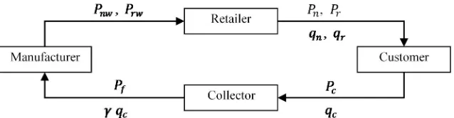
Figure 1. Framework of the closed-loop pricing model with random yield
The product considered in this model is single item, short life-cycle, with obsolescence effect after a certain period, in term of obsolescence in function and desirability. Demands are random, with time-dependent functions which represent the short life-cycle pattern along the entire phases of product life-cycle, both for new and remanufactured products; and linear in price.
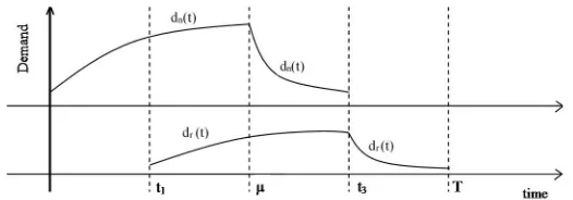
There are four time frames considered in this model, as depicted in Figure 2. In the first interval [0, t1], only new product is offered to the market. In second and third interval,i.e. [t1, ] and[, t3], both new and remanufactured products are offered. The difference between second and third interval is on the segments of life-cycle phases for both types. During second interval, both new and remanufactured products are at the IMG phases.In the third interval, the new product has entered the decline phase while remanufactured product has not. In the fourth interval [t3, T], manufacturer has stopped producing new product and only offers remanufactured product which is assumed to be on the decline phase.
The market demand capacity is adopted from (Wang & Tung 2011) and extended to cover the obsolescence period, where demand decreases significantly. The demand patterns are constructed for both new and remanufactured product and the governing functions are formulated as follows:
seen in Figure 2. U is a parameter representing the maximum possible demand for new product, is the time when the demand reaches its peak, i.e. at U level. d0 is the demand at the beginning of the life-cycle (when t = 0), and λ is the speed of change in the demand as a function of time. A parallel definition is applicable for V, t3, dr0, and η respectively for the remanufactured products. It
is obvious that dn(t) and dr(t) are continuous at and t3, respectively.
Since demand of new and remanufactured products are random and both depend on the price of new product as well as the price of remanufactured product, the demand functions can be expressed as
( , , ) = ( ) ( 1− + )∙ ………(3.3)
( , , ) = ( ) ( 1− + )∙ ………(3.4)
575
Figure 2. Demand pattern of a product with gradual obsolescence, over time
The demand function information is shared to all members of the supply chain. The pricing game mechanism is started with manufacturer as the Stackelberg leader releasing wholesale prices. This information is used by retailer, along with observation to the market demand, to decide the optimal retail prices as well as the order quantities. Collector, on the other hand, observes the demand of remanufactured product and decides the optimal acquisition price, while considering the random yield factor. The remanufacturable acquired products are then transferred to the manufacturer, who further decides the wholesale prices for both new and remanufactured products.
4. OPTIMIZATION 4.1Retailer’s optimization
Manufacturer makes the first move by releasing initial wholesale prices and . Retailer then optimizes the retail prices under sequential approach:
Optim1: max , Π ( , ) |( ∗ , ∗ ) = ∗ ( − ) + ∗ ( − ) ………(4.1)
where ( ∗ , ∗ ) is the solution of Optim2
Optim2a:max , Π ( , ) |( , ) = max
, [ ∙min( ( ) , ) ] +
[ ∙min( ( ) , ) ] − −
………(4.2)
where ( ) is the total demand over [0, ] for new products, a function of random variable ; and ( ) is the total demand over [ ,T] for remanufactured products, a function of random variable .
Therefore,
( ) = ∫ ( 1− + ) ∙ + ∫
( ) ( 1− + )∙ =
( 1− + ) ∙ ………
(4.3)
( ) = ∫ ( )( 1− + )∙ + ∫
( ) ( 1− + )∙ =
( 1− + ) ∙ ……… (4.4)
where
=
( )
( )
……… (4.5)
=
( ) ( )
( )
……… (4.6)
At somegiven prices and , the expected quantities that maximize profit can be found by first letting =
576
and =
( ) , the value of random variable when ( ) = ; these are similar to the
stocking factor proposed by Li et al. (2009).
[ ∙min( ( ) , ) ] = ∙ [ min( ( ) , ) ]= ∙ ∫ ( ) ( ) + ∫ ( ) =
∙ ∫ ( ) ( ) + ( )
Similarly, [ ∙min( ( ) , ) ] = ∙ ∫ ( ) ( ) + ̅( )
where ( ) = 1− ( ) and ̅( ) = 1− ( )
The optimization problem becomes Optim2b:
max , Π = max
,, ∙ ∫
( ) ( ) + ( ) − + ∙
∫ ( ) ( ) + ̅( ) −
……… (4.7)
Since =
( ) and = ( ) , then
Π
= ∙ ( ) ( )
( ) + ( ) −
( )
( ) − = 0 ……… (4.8)
Π
= ∙ ( ) ( )
( ) + ̅( ) −
( )
( ) − = 0 ……… (4.9)
Simplifying the equations, we find
( ) = ……… (4.10)
̅
( ) = ……… (4.11)
so the optimal quantities are ∗ , ∗ where
∗ = ( 1− + ) ……… (4.12)
∗ = ( 1− + ) ̅ ……… (4.13)
Now we find optimal prices by solving Optim1
max , Π ( , ) |( ∗ , ∗ ) = ( 1− + ) ( − ) + ( 1− +
) ̅ ( − ) ……… (4.14)
Π
=
( 1−2 + + ) +
( 1− + ) ( − ) + ̅ ( − ) = 0
……… (4.15)
Π
= ( 1−2 + + ) ̅ +
( 1− + ) ( − ) ̅ + ( − ) = 0
……… (4.16)
577
4.2 Collector’s Optimization
The collector problem is significantly influenced by the random yield factor,since only a portion ( )of returned used product meets the input requirements to the remanufacturing process. The quantity of returns, , is influenced by acquisition price, ; which approach has been used in several studies such asQiaolun et al. (2008)andLi et al. (2009). Collector performs inspection and sorting tothe acquired returns, and transfers the remanufacturable items to the manufacturer at a transfer price . Returns that do not meet the quality requirement are disposed. Since the collector decides on collected quantity before random yield factor is realized, the quantity of remanufacturable items can be higher or lower than the manufacturer’s order quantity( ). Therefore, shortage penalty( )and salvage value( ) are applied to the model. Yield factor is a random variable with density function ℎ( ) and cumulative distribution function ( ).
The governing equation for collection quantity as a function of collection price is given as
= Θ( ) = , ……… (4.17)
similar to the return rate used inQiaolun et al. (2008), where is a positive constant coefficient and
[0,1] is the exponent of thepower function, which determine the curve’s steepness. The collector’s optimization problem can be expressed as
Optim3a: max Π ( ) = ∙ [ min( , )− [ − ] + [ − ] ]− ( + )
……… (4.18) Let = , which represents the value of when = ; and replace with
according to the collection function, optimization problem Optim3 becomes
max Π ( ) = + − ∫ ( − )ℎ( ) + − + ( ) −
+ ……… (4.19)
Applying the first derivative condition, we find
Π
= + − ( − )ℎ( ) + ∫ ℎ( ) + ( ) − 1 + −
= 0 ……… (4.20)
Since = and = − ,
+ − ∫ ℎ( ) + ( ) − 1 + − = 0 ……… (4.21)
The optimal collection quantityis ∗ that satisfies equation (4.21)and ∗ = ∗ .
These optimums depends on yield factor randomness, parameters in collection function, order quantity of remanufactured product, transfer price and shortage penalty as well as salvage value.
4.2 Manufacturer’ Optimization
578
Optim4a: max , Π = ( − − ) + min( , ) ∙ − − −
[ − ] ……… (4.22)
where and are unit raw material cost and unit manufacturing cost for new product, while is remanufacturing cost and is unit shortage penalty.
Since retailer’s optimal quantities are given as in (4.12) and (4.13), the optimization problem becomes
Optim4b:
max , Π = ( 1− + ) ( − − ) +
min ( 1− + ) ̅ , ∙ − − −
( 1− + ) ̅ −
……… (4.23)
Let = ( 1− + ), = ( 1− + ); Φ( ) = ( ), and Ψ( ) = ̅ ( ) with
their first derivativesΦ′( ) = ( ) and Ψ′( ) = ̅ ( ) .
Also, let =
( ) ̅
= Ψ , which represents the value of random yield factor when = . Therefore, the optimization problem can be expressed as follow
Optim4c: max , Π = Φ ( − − ) + − − +
− − + ∫ ( − ) ( ) ……… (4.24)
Since is a function of , taking first derivative to can be done by applying chain rule, with
= . Therefore, the first derivative conditions are
(1) = Φ ( − − ) + Φ = 0 ……… (4.25)
(2) = − − + + ∫ ( − )ℎ( ) + − − +
∫ ( − )ℎ( ) = 0 ……… (4.26)
which can be simplified into
1
Ψ − − ( ) + ( ) + + ( − )ℎ( )
= 0
……… (4.27) The optimal wholesale prices are ∗ that satisfies (4.25) and ∗ that satisfies (4.27).
579
5. NUMERICAL EXAMPLE
The pricing decision problem in this numerical example involves the following parameters: price sensitiveness for demands of new and remanufactured product = 0.003, = 0.0001, = 0,004, = 0,0002. The demand capacity of new product contains parameters , , such that
= 4000, while demand capacity of remanufactured product has parameters , , such that
= 1500. The unit raw material cost for new product = 50, unit manufacturing cost
= 40, unit remanufacturing cost = 20, and unit collecting cost = 4. Parameters in the return rate function are = 0.1 and = 0.7. Collector’s shortage penalty and salvage value are
= 5and = 8 respectively. Manufacturer’s shortage penalty is = 50. Transfer price is
= 40. The initial wholesale prices releases by manufacturer are = 120 and = 80, for new and remanufactured product. , , are random variables with uniform distribution on finite support [0,1].
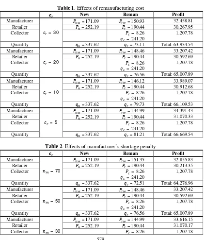
Table 1. Effects of remanufacturing cost
New Reman Profit
Table 2. Effects of manufacturer’s shortage penalty
580
= 241.20
Quantity =337.62 =81.21 Total: 65,894.10
Manufacturer
= 10
=171.09 =140.65 3,4391.43
Retailer =252.19 =190.44 31,692.54
Collector = 8.26
= 241.20
1,207.78
Quantity =337.62 =86.64 Total: 67,001.09
The optimization problems are solved using Matlab. Then, we perform sensitivity analysis for several factors that are important to the pricing decision, which are unit remanufacturing cost, manufacturer’s shortage penalty, and the parameters of random yield. We use uniform distribution for random variables in the demand functions as well as the yield factor. The results are shown in Tables 1 – 4.
Table 1 shows that an increase in remanufacturing cost would lower the profit of retailer and manufacturer, while the collector’s profit is not affected by it. Remanufacturing cost does not affect retailer’s and collector’s pricing decision, as expected from the analytical model, but it affects the wholesale price of remanufactured product. As remanufacturing cost increases, manufacturer responds to it by increasing the wholesale price instead of the decreasing effect in the quantity.Therefore, both retailer and manufacturer get lower profit, even though manufacturer’s profit drops twice as fast as retailer’s.
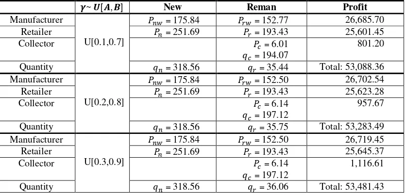
Table 3. Effects of the mean value of the random yield
~ [ , ] New Reman Profit
Manufacturer
U[0.1,0.7]
=175.84 =152.77 26,685.70
Retailer =251.69 =193.43 25,601.45
Collector =6.01
=194.07
801.20
Quantity =318.56 =35.44 Total: 53,088.36
Manufacturer
U[0.2,0.8]
=175.84 =152.50 26,702.54
Retailer =251.69 =193.43 25,623.28
Collector =6.14
=197.12
957.67
Quantity =318.56 =35.75 Total: 53,283.49
Manufacturer
U[0.3,0.9]
=175.84 =152.50 26,719.45
Retailer =251.69 =193.43 25,645.37
Collector =6.14
=197.12
1,116.61
Quantity =318.56 =36.06 Total: 53,481.43
Table 4. Effects of variance in the random yield
~ [ , ] New Reman Profit
Manufacturer
U[0.2,0.8]
=175.84 =152.50 26,702.54
Retailer =251.69 =193.43 25,623.28
Collector =6.14
=197.12
957.67
Quantity =318.56 =35.75 Total: 53,283.49
Manufacturer =175.84 =149.23 26,914.92
581
Collector U[0.1,0.9] =5.45
=181.25
1,723.15
Quantity =318.56 =39.66 Total: 54,551.40
Manufacturer
U[0,1]
=175.84 =146.94 27,067.62
Retailer =251.69 =193.43 26,138.30
Collector =4.97
=203.44
2,218.29
Quantity =318.56 =42.55 Total: 55,424.21
Similarly, as shown in Table 2, when manufacturer’s shortage penalty increases, retailer’s and manufacturer’s profit decrease, while collector’s profit is again not affected. Manufacturer reacts by increasing the wholesale price of remanufactured product to cover the risk of receiving shortage penalty, and in turns decreasing the quantity of remanufactured product. While both manufacturer and retailer hurts by receiving lower profit, this time retailer’s profit drops slightly faster than manufacturer’s.
The shift in mean value of random yield influence the profit received by all three parties in positive direction as given in Table 3. As the expected value of random yield gets higher, there would be a bigger portion of collected used products that meet remanufacturing requirement. Hence, the probability to supply lower than the order quantity decreases, and total quantity of remanufactured product increases. Collection price also increases to increase the collection quantity, as a respond to higher order quantity of remanufactured product. All members’ profits increase as the expected value for random yield increases as a result of order fulfillment and less penalties. Collector’s percentage profit increase is significantly higher than the others because yield factor of product returns is harbored in collector’s inspection and sorting process.Similar argument applies for the variance of random yield, as shown in Table 4.It is interesting that an increase in variance of random yield is responded by lowering wholesale price and collection price, and this actions increase the remanufactured product’s quantity which in turn increase the supply chain profit. However, the decrease in wholesale and collection prices as the variance of random yield gets higher, is more notable than that in mean value’s effect. We find that wholesale price of remanufactured product and collection price are more robust to a shift in mean value of random yield rather than a change in random yield’s variance.
5 CONCLUSION
Pricing decision problem in a closed-loop supply chain with remanufacturing under random yield and random demand is an important problem that needs to be addressed because it significantly affects profitability. Unlike many previous studies that consider one member of the supply chain, we develop a model that involves three key members of the supply chain, namely manufacturer, retailer and collector; for a short life cycle product.
The results show that remanufacturing cost and manufacturer’s shortage penalty influence the wholesale price of the remanufactured product and further has impact on the retailer’s and manufacturer’s profit. A decrease in remanufacturing cost and manufacturer’s shortage penalty increase the total profit. On the other hand the mean value and variance of random yield has positive effect in the supply chain’s profit, as the higher the mean value and the variance, the higher the profit of each of the member.We also find that wholesale price of remanufactured product is more robust to a shift in mean value of random yield rather than a change in random yield’s variance.
582
Atasu, A., Guide, V.D.R.J. & Wassenhove, L.N. Van, 2010. So what if remanufacturing cannibalizes my new product sales? California Management Review, 52(2), pp.56–76.
Atasu, A., Sarvary, M. & Wassenhove, L.N. Van, 2008. Remanufacturing as a marketing strategy. Management Science, 54(10), pp.1731–1746.
Bakal, I.S. & Akcali, E., 2006. Effects of Random Yield in Remanufacturing with Price-Sensitive Supply and Demand. Production and Operations Management, 15(3), pp.407–420.
Ferguson, M.E. et al., 2009. The Value of Quality Grading in Remanufacturing. Production and Operations Management, 18(3), pp.300–314.
Ferrer, G. & Guide, V.D.R.J., 2002. Remanufacturing cases and state of the art. In R. U. Ayres & L. W. Ayres, eds. A handbook of industrial ecology. Chelten-ham: Edward Elgar Publishing, pp. 510–520. Ferrer, G. & Swaminathan, J.M., 2006. Managing New and Remanufactured Products. Management
Science, 52(1), pp.15–26.
Guide, V.D.R.J., Muyldermans, L. & Wassenhove, L.N. Van, 2005. Hewlett-Packard Company Unlocks the Value Potential from Time-Sensitive Returns. Interfaces, 35(4), pp.281–293.
Guide, V.D.R.J., Teunter, R.H. & Wassenhove, L.N. Van, 2003. Matching Demand and Supply to Maximize Profits from Remanufacturing. Manufacturing & Service Operations Management, 5(4), pp.303–316.
Guide, V.D.R.J. & Wassenhove, L.N. Van, 2009. The Evolution of Closed-Loop Supply Chain Research. Operations Research, 57(1), pp.10–18.
Jena, S.K. & Sarmah, S.P., 2013. Optimal acquisition price management in a remanufacturing system. International Journal of Sustainable Engineering.
Li, X., Li, Y. & Cai, X., 2009. Collection Pricing Decision in a Remanufacturing System Considering Random Yield and Random Demand. Systems Engineering - Theory & Practice, 29(8), pp.19–27. Li, X., Li, Y. & Cai, X., 2014. Remanufacturing and pricing decisions with random yield and random
demand. Computers & Operations Research, pp.1–9. Available at: http://dx.doi.org/10.1016/j.cor.2014.01.005.
Liang, Y., Pokharel, S. & Lim, G.H., 2009. Pricing used products for remanufacturing. European Journal of Operational Research, 193(2), pp.390–395.
Lund, R.T. & Hauser, W.M., 2009. Remanufacturing – An American Perspective,
Mukhopadhyay, S.K. & Ma, H., 2009. Joint procurement and production decisions in remanufacturing under quality and demand uncertainty. International Journal of Production Economics, 120(1), pp.5– 17.
Ovchinnikov, A., 2011. Revenue and Cost Management for Remanufactured Products. Production and Operations Management, 20(6), pp.824–840.
Qiang, Q. et al., 2013. The closed-loop supply chain network with competition, distribution channel investment, and uncertainties. Omega, 41(2), pp.186–194.
Qiaolun, G., Jianhua, J. & Tiegang, G., 2008. Pricing management for a closed-loop supply chain. Journal of Revenue and Pricing Management, 7(1), pp.45–60.
Robotis, A., Boyaci, T. & Verter, V., 2012. Investing in reusability of products of uncertain remanufacturing cost: The role of inspection capabilities. International Journal of Production Economics, 140(1), pp.385–395.
Seitz, M.A., 2007. A critical assessment of motives for product recovery: the case of engine remanufacturing. Journal of Cleaner Production, 15, pp.1147–1157.
Souza, G.C., 2013. Closed-Loop Supply Chains: A Critical Review, and Future Research. Decision Sciences, 44(1), pp.7–38.
Teunter, R.H. & Flapper, S.D.P., 2011. Optimal core acquisition and remanufacturing policies under uncertain core quality fractions. European Journal of Operational Research, 210, pp.241–248.
Wang, K.-H. & Tung, C.-T., 2011. Construction of a model towards EOQ and pricing strategy for gradually obsolescent products. Applied Mathematics and Computation, 217(16), pp.6926–6933. Wei, J. & Zhao, J., 2011. Pricing decisions with retail competition in a fuzzy closed-loop supply chain.
583
Wu, C.-H., 2013. OEM product design in a price competition with remanufactured product. Omega, 41, pp.287–298.