The Finite Difference Method
10.1
Hyperbolic Equations
Wave Equation
As an example of a hyperbolic partial differential equation, we consider the wave equa-tion
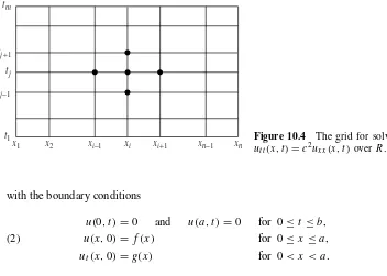
tm
The wave equation models the displacementuof a vibrating elastic string with fixed ends at x = 0 and x = a. Although analytic solutions to the wave equation can be obtained with Fourier series, we use the problem as a prototype of a hyperbolic equation.
Derivation of the Difference Equation
Partition the rectangle R = {(x,t): 0≤ x ≤a,0≤t ≤ b}into a grid consisting of
n−1 bym−1 rectangles with sidesx =handt =k, as shown in Figure 10.4. Start at the bottom row, wheret =t1=0 and the solution is known to beu(xi,t1)= f(xi).
We shall use a difference-equation method to compute approximations
r2 u
which in turn are substituted into (1); this produces the difference equation
(5) ui,j+1−2ui,j +ui,j−1
k2 =c
2ui+1,j−2ui,j +ui−1,j
h2 ,
which approximates equation (1). For convenience, the substitutionr =ck/his intro-duced in (5), and we obtain the relation
(6) ui,j+1−2ui,j +ui,j−1=r2(ui+1,j −2ui,j +ui−1,j).
Equation (6) is employed to find row j +1 across the grid, assuming that approxima-tions in both rows j and j −1 are known:
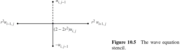
(7) ui,j+1=(2−2r2)ui,j +r2(ui+1,j +ui−1,j)−ui,j−1,
fori =2, 3,. . .,n−1. The four known values on the right side of equation (7), which are used to create the approximationui,j+1, are shown in Figure 10.5.
Caution must be taken when using formula (7). If the error made at one stage of the calculations is eventually dampened out, the method is calledstable. To guarantee stability in formula (7), it is necessary thatr = ck/h ≤ 1. There are other schemes, calledimplicitmethods, that are more complicated to implement, but do not have sta-bility restrictions forr.
Starting Values
Two starting rows of values corresponding to j = 1 and j = 2 must be supplied in order to use formula (7) to compute the third row. Since the second row is not usually given, the boundary functiong(x)is used to help produce starting approximations in the second row. Fixx = xi at the boundary and apply Taylor’s formula of order 1 for
expandingu(x,t)about(xi,0). The valueu(xi,k)satisfies
Then use u(xi,0) = f(xi) = fi andut(xi,0) = g(xi) = gi in (8) to produce the
formula for computing the numerical approximations in the second row:
(9) ui,2= fi +kgi for i =2, 3, . . ., n−1.
Usually, u(xi,t2) = ui,2, and such errors introduced by formula (9) will propagate throughout the grid and will not be dampened out when the scheme in (7) is imple-mented. Hence it is prudent to use a very small step size fork so that the values for
ui,2given in (9) do not contain a large amount of truncation error.
Often, the boundary function f(x)has a second derivative f′′(x)over the interval. In this case we haveux x(x,0)= f′′(x), and it is beneficial to use the Taylor formula
of ordern = 2 to help construct the second row. To do this, we go back to the wave equation and use the relationship between the second-order partial derivatives to obtain
(10) ut t(xi,0)=c2ux x(xi,0)=c2f′′(xi)=c2fi+1−2fi + fi−1
Usingr =ck/h, formula (12) can be simplified to obtain a difference formula for the improved numerical approximations in the second row:
The French mathematician Jean Le Rond d’Alembert (1717–1783) discovered that
(14) u(x,t)=F(x+ct)+G(x−ct)
is a solution to the wave equation (1) over the interval 0 ≤ x ≤ a, provided that
F′, F′′, G′, andG′′ all exist and FandG have period 2aand obey the relationships
allz. We can check this out by direct substitution. The second-order partial derivatives
Substitution of these quantities into (1) produces the desired relationship:
ut t(x,t)=c2F′′(x+ct)+c2G′′(x−ct)
The accuracy of the numerical approximations produced by the equations in (7) de-pends on the truncation errors in the formulas used to convert the partial differential equation into a difference equation. Although it is unlikely to know values of the exact solution for the second row of the grid, if such knowledge were available, using the incrementk=chalong thet-axis will generate an exact solution at all the other points throughout the grid.
Theorem 10.1. Assume that the two rows of values ui,1 = u(xi,0) andui,2 =
u(xi,k), fori = 1, 2,. . .,n, are the exact solutions to the wave equation (1). If the step sizek=h/cis chosen along thet-axis, thenr =1 and formula (7) becomes
(17) ui,j+1=ui+1,j +ui−1,j −ui,j−1.
Furthermore, the finite-difference solutions produced by (17) throughout the grid are exact solution values to the differential equation (neglecting computer round-off error).
Proof. Use d’Alembert’s solution and the relationck=h. The calculationxi−ctj =
(i−1)h−c(j−1)k=(i −1)h−(j−1)h=(i− j)hand a similar one producing
xi+ctj =(i+j−2)hare used in equation (14) to produce the following special form
ofui,j:
(18) ui,j =F((i− j)h)+G((i+ j −2)h)
ui+1,j,ui−1,j, andui,j−1on the right side of (17) yields
Warning. Theorem 10.1 does not guarantee that the numerical solutions are exact when numerical calculations based on (9) and (13) are used to construct approxima-tions ui,2 in the second row. Indeed, truncation error will be introduced if ui,2 =
u(xi,k) for somei, where 1 ≤ i ≤ n. This is why we endeavor to obtain the best
possible values for the second row by using the second-order Taylor approximations in equation (13).
Example 10.1. Use the finite-difference method to solve the wave equation for a vibrating string: Substitutingr=1 into equation (7) gives the simplified difference equation (22) ui,j+1=ui+1,j+ui−1,j−ui,j−1.
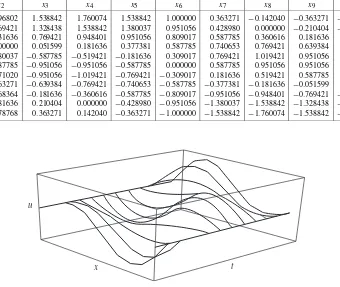
Applying formulas (21) and (22) successively to generate rows will produce the approxi-mations tou(x,t)given in Table 10.1 for 0<xi <1 and 0≤tj ≤0.50.
The numerical values in Table 10.1 agree to more than six decimal places of accuracy with those obtained with the analytic solution
Table 10.1 Solution of the Wave Equation (19) with Boundary Conditions (20)
tj x2 x3 x4 x5 x6 x7 x8 x9 x10
0.00 0.896802 1.538842 1.760074 1.538842 1.000000 0.363271 −0.142040 −0.363271 −0.278768 0.05 0.769421 1.328438 1.538842 1.380037 0.951056 0.428980 0.000000 −0.210404 −0.181636 0.10 0.431636 0.769421 0.948401 0.951056 0.809017 0.587785 0.360616 0.181636 0.068364 0.15 0.000000 0.051599 0.181636 0.377381 0.587785 0.740653 0.769421 0.639384 0.363271 0.20 −0.380037 −0.587785 −0.519421 −0.181636 0.309017 0.769421 1.019421 0.951056 0.571020 0.25 −0.587785 −0.951056 −0.951056 −0.587785 0.000000 0.587785 0.951056 0.951056 0.587785 0.30 −0.571020 −0.951056 −1.019421 −0.769421 −0.309017 0.181636 0.519421 0.587785 0.380037 0.35 −0.363271 −0.639384 −0.769421 −0.740653 −0.587785 −0.377381 −0.181636 −0.051599 0.000000 0.40 −0.068364 −0.181636 −0.360616 −0.587785 −0.809017 −0.951056 −0.948401 −0.769421 −0.431636 0.45 0.181636 0.210404 0.000000 −0.428980 −0.951056 −1.380037 −1.538842 −1.328438 −0.769421 0.50 0.278768 0.363271 0.142040 −0.363271 −1.000000 −1.538842 −1.760074 −1.538842 −0.896802
u
x t
Figure 10.6 The vibrating string for equations (19) and (20).
A three-dimensional presentation of the data in Table 10.1 is given in Figure 10.6.
Example 10.2. Use the finite-difference method to solve the wave equation for a vibrating string:
(23) ut t(x,t)=4ux x(x,t) for 0<x<1 and 0<t <0.5,
with the boundary conditions
(24)
u(0,t)=0 and u(1,t)=0 for 0≤t ≤1, u(x,0)= f(x)=
x for 0≤x≤ 35
1.5−1.5x for 35 ≤x≤1, ut(x,0)=g(x)=0 for 0<x<1.
Table 10.2 Solution of the Wave Equation (23) with Boundary Conditions (24)
tj x2 x3 x4 x5 x6 x7 x8 x9 x10
0.00 0.100 0.200 0.300 0.400 0.500 0.600 0.450 0.300 0.150
0.05 0.100 0.200 0.300 0.400 0.500 0.475 0.450 0.300 0.150
0.10 0.100 0.200 0.300 0.400 0.375 0.350 0.325 0.300 0.150
0.15 0.100 0.200 0.300 0.275 0.250 0.225 0.200 0.175 0.150
0.20 0.100 0.200 0.175 0.150 0.125 0.100 0.075 0.050 0.025
0.25 0.100 0.075 0.050 0.025 0.000 −0.025 −0.050 −0.075 −0.100
0.30 −0.025 −0.050 −0.075 −0.100 −0.125 −0.150 −0.175 −0.200 −0.100
0.35 −0.150 −0.175 −0.200 −0.225 −0.250 −0.275 −0.300 −0.200 −0.100
0.40 −0.150 −0.300 −0.325 −0.350 −0.375 −0.400 −0.300 −0.200 −0.100
0.45 −0.150 −0.300 −0.450 −0.475 −0.500 −0.400 −0.300 −0.200 −0.100
0.50 −0.150 −0.300 −0.450 −0.600 −0.500 −0.400 −0.300 −0.200 −0.100
u
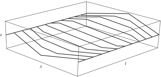
x t
Figure 10.7 The vibrating string for equations (23) and (24).
approximations tou(x,t)given in Table 10.2 for 0≤xi ≤1 and 0≤tj ≤0.50. A