Dynamic Effects of Social Influence and Direct Marketing on the Adoption of High-Technology Products

Hans Risselada, Peter C. Verhoef, & Tammo H.A. Bijmolt

Dynamic Effects of Social Influence

and Direct Marketing on the

Adoption of High-Technology

Products

Many firms capitalize on their customers’ social networks to improve the success rate of their new products. In this article, the authors analyze the dynamic effects of social influence and direct marketing on the adoption of a new high-technology product. Social influence is likely to play a role because the decision to adopt a high-involvement product requires extensive information gathering from various sources. The authors use call detail records to construct ego networks for a large sample of customers of a Dutch mobile telecommunications operator. Using a fractional polynomial hazard approach to model adoption timing and multiple social influence variables, they provide a fine-grained analysis of social influence. They show that the effect of social influence from cumulative adoptions in a customer’s network decreases from the product introduction onward, whereas the influence of recent adoptions remains constant. The effect of direct marketing is also positive and decreases from the product introduction onward. This study provides new insights into the adoption of high-technology products by analyzing dynamic effects of social influence and direct marketing simultaneously.

Keywords: adoption, social influence, dynamic modeling, high-technology products

Hans Risselada is Assistant Professor of Marketing (e-mail: H.Risselada@ rug.nl), and Tammo H.A. Bijmolt is Professor of Marketing Research (e-mail: T.H.A.Bijmolt@rug.nl), Faculty of Economics and Business, University of Groningen. Peter C. Verhoef is Professor of Marketing, Faculty of Econom-ics and Business, University of Groningen, and Research Professor in Marketing, BI Norwegian Business School (e-mail: P.C.Verhoef@rug.nl). The authors acknowledge an anonymous Dutch telecommunications operator for providing the data. They thank TNO, the Dutch Research Delta, and the Customer Insights Center at University of Groningen for supporting this research as well as Jenny van Doorn, Maarten Gijsenberg, and Sander Beckers for their helpful comments on earlier versions of this article. They are also grateful to participants of the KU Leuven Winter Camp 2010, Marketing Science Conference in Cologne 2010, Marketing Dynamics Conference in Istanbul 2010, and Erasmus School of Econom-ics 2013. Finally, the authors thank three anonymous JMreviewers for their helpful comments. Peter Danaher served as area editor for this article.

T

he effectiveness of traditional marketing instruments

has declined in many markets, whereas the effects of social interactions between consumers on buying behavior and the opportunities to exploit these interactions have increased (Sethuraman, Tellis, and Briesch 2011; Van den Bulte and Wuyts 2007). As a result, marketers have shown renewed interest in the effects of social influence or social contagion on customer behavior (Kumar, Petersen, and Leone 2007; Van den Bulte and Wuyts 2007). The increasing prevalence of social media, such as Facebook and LinkedIn, has created an even stronger interest in social influence effects. These developments pose new challenges for marketing researchers and practitioners (Godes and Mayzlin 2004; Libai et al. 2010; Stephen and Galak 2012).

In this article, we specifically address social influence effects on adoption of high-technology products.

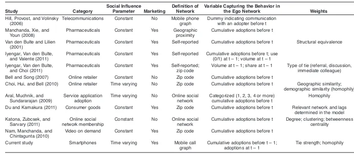
Table 1 provides a selective overview of the extant lit-erature on the impact of social influence on the adoption process. Prior research has revealed a positive effect of social influence on adoption in multiple industries, includ-ing telecommunications (Hill, Provost, and Volinsky 2006), online retailing (Bell and Song 2007; Choi, Hui, and Bell 2010), and pharmaceuticals (Iyengar, Van den Bulte, and Valente 2011). Although studies on this main effect of social influence provide valuable insights, several issues remain relatively unexplored.

Dy

na

m

ic

E

ffe

ct

s

of

S

oc

ia

l Inf

lue

nc

e

and

Di

re

ct

M

ar

ke

ting

/ 5

3

Study Category

Social Influence

Parameter Marketing

Definition of Network

Variable Capturing the Behavior in

the Ego Network Weights

Hill, Provost, and Volinsky (2006)

Telecommunications Constant No Mobile phone

graph

Dummy indicating communication with an adopter before t Manchanda, Xie, and

Youn (2008)

Pharmaceuticals Constant Yes Geographic

proximity

Cumulative adoptions before t

Van den Bulte and Lilien (2001)

Pharmaceuticals Constant Yes Self-reported Cumulative adoptions before t Structural equivalence

Iyengar, Van den Bulte, and Valente (2011)

Pharmaceuticals Constant Yes Self-reported Cumulative adoptions before t; use (0/1) at t – 1; volume at t – 1 Iyengar, Van den Bulte,

and Choi (2011)

Pharmaceuticals Constant Yes Self-reported;

zip code

Volume at t – 1; share at t – 1 Type of tie (referral, discussion, immediate colleague)

Bell and Song (2007) Online retailer Constant No Zip code Cumulative adoptions before t

Choi, Hui, and Bell (2010) Online retailer Time varying No Zip code Cumulative adoptions before t Geographic similarity; demographic similarity (homophily) Aral, Muchnik, and

Sundararajan (2009)

Service application adoption

Time varying No Online social

network

Categorized (1, 2, 3, 4 or more) cumulative adoptions before t

Homophily

Du and Kamakura (2011) Consumer goods Constant Yes Zip code Cumulative adoptions before t Relevant network and lags

determined in the model Katona, Zubcsek, and

Sarvary (2011)

Online social network membership

Constant No Online social

network

Cumulative adoptions before t Degree; clustering; betweenness centrality

Nam, Manchanda, and Chintagunta (2010)

Video on demand Constant Yes Zip code Cumulative adoptions before t

Current study Smartphones Time varying Yes Mobile call

graph

Cumulative adoptions before t – 1; adoptions at t – 1

Tie strength; homophily TABLE 1

Second, prior research on social influence effects on adoption has distinguished the effects of recent adoptions (e.g., Hill, Provost, and Volinsky 2006; Iyengar, Van den Bulte, and Choi 2011) and cumulative adoptions (e.g., Katona, Zubcsek, and Sarvary 2011) in a person’s network. Recent and cumulative measures for social influence cover theoretically separate contagion processes. Recent adopters may be more contagious than consumers who adopted less recently because they are more enthusiastic or credible (Iyengar, Van den Bulte, and Valente 2011). The cumulative adoption term might signal which behavior has become the norm in a person’s network. The majority of studies have, however, focused on the effects of cumulative adoptions (see Table 1). In addition, the effects of recent and cumula-tive adoptions may vary over time. This study is the first that simultaneously considers the effects of recent and cumulative adoptions in a person’s network on adoption over time.

Third, several social network metrics have been dis-cussed within the social network literature stream. Tie strength is a variable that has received considerable atten-tion in the marketing and adopatten-tion literature streams (e.g., Iyengar, Van den Bulte, and Choi 2011; Reingen and Ker-nan 1986). Only recently have studies also considered the role of homophily (see Table 1), which involves the similar-ity between a customer and his or her network (e.g., Choi, Hui, and Bell 2010; Nitzan and Libai 2011). In this study, we account both for tie strength and homophily when studying social influence effects because these social influ-ence variables may have differential effects.

Fourth, an important discussion in the literature is whether social influence exists when researchers control for marketing efforts. Studies on social influence have fre-quently ignored marketing-mix effects, which might cause the effects of social influence to be biased upward because of so-called correlated effects (Manski 2000; Van den Bulte and Lilien 2001). Only two studies, both in a pharmaceuti-cal context, have examined marketing and social influence effects at the individual level (Iyengar, Van den Bulte, and Valente 2011; Manchanda, Xie, and Youn 2008). In this study, we simultaneously assess the effects of direct mar-keting and social influence on the adoption of a new prod-uct to further establish whether social influence effects in a consumer context remain present when researchers account for the role of marketing.

This discussion leads us to ask the following two research questions: (1) What are the effects of social influ-ence variables—in particular, recent and cumulative adop-tions—on the adoption of a new product when accounting for the effect of direct marketing? and (2) How do these effects and the effect of direct marketing change from the product introduction onward? Thus, this study contributes to the literature by providing fine-grained insights on the effects of social influence on adoption over time, namely, that (1) the effect of social influence from recent adoptions is positive and constant from the product introduction onward, (2) the effect of cumulative adoptions is positive and decreases from the product introduction onward, and

(3) the effect of direct marketing is positive and decreases from the product introduction onward.

The remainder of this article is structured as follows: We begin with a discussion of our conceptual background. Next, we describe our conceptual model and formulate our hypotheses. We then present our data. We use individual-level data on smartphone adoption, customer characteristics (e.g., service usage, gender), direct marketing efforts, and call detail records (CDRs) of a random sample of customers of a major Dutch mobile telecommunications operator. Next, we elaborate on the econometric model. We analyze the time-varying effects of social influence and marketing on individ-ual adoption behavior using a hazard model with a fractional polynomial approach (Berger, Schäfer, and Ulm 2003; Royston and Altman 1994). In the next section, we provide an overview of the results, addressing the aforementioned research questions. Finally, we discuss the main findings and offer management implications and study limitations.

Conceptual Model and Hypotheses

The marketing literature, and specifically the new product diffusion literature, has acknowledged the important role of social influence or contagion for decades. We define social influence as the effect of an adoption in a customer’s net-work of any smartphone at the focal company on the smart-phone adoption probability of that customer. It is important to distinguish this approach to social influence from the one frequently used in the social psychology literature, in which the focus is on the underlying persuasion processes (e.g., Cialdini 2007). In this article, we do not adopt a social psy-chological view and instead focus on the marketing litera-ture on social contagion and networks (e.g., Van den Bulte 2010; Van den Bulte and Stremersch 2004). Consequently, we do not unravel the processes and mechanisms that drive the influence, such as compliance, identification, or inter-nalization (Kelman 1958).

The traditional Bass (1969) model considers two impor-tant factors in the diffusion process with its parameters p and q, where p is the innovation parameter and q is the con-tagion parameter. Concon-tagion exists as a result of several theoretical mechanisms, such as social learning under uncertainty, social normative pressures, competitive con-cerns, and performance network effects (Van den Bulte and Lilien 2001; Van den Bulte and Stremersch 2004). How-ever, in their meta-analysis on the size of the p and q parameters, Van den Bulte and Stremersch (2004, p. 542) conclude that contagion may not be as important as it is commonly believed to be. For example, Van den Bulte and Lilien (2001) find that contagion effects may disappear when marketing is accounted for.

investi-gated contagion effects at the individual level because there is an absence of network data. Only recently have we observed an increase in studies investigating social influ-ence effects at the individual level (e.g., Choi, Hui, and Bell 2010; Iyengar, Van den Bulte, and Valente 2011). Some researchers have concluded that the existence of social influence effects at the individual level are now established (Godes 2011). However, Van den Bulte and Iyengar (2011) show that these effects are not clear and straightforward because previous studies involve incorrect models and data. Adoption by consumers in the network can affect the focal consumer in two ways. First, the awareness that a spe-cific number of consumers have adopted the product in the past leads to a general buzz type of social influence. Sec-ond, new adoptions may directly affect the consumer (e.g., by communication about the new product or imitation). Therefore, when studying social influence on adoption, researchers must consider both recent adoption behavior and past cumulative adoption behavior in a network. In a pharmaceutical context, Iyengar, Van den Bulte, and Valente (2011) show a significant effect of prescription volume at t – 1, whereas the effect of cumulative adoptions is not sig-nificant. In this study, we account for both types of social influence: recent adoptions in a network at time t – 1 and cumulative adoptions in a person’s network before t – 1.

The social network literature stream distinguishes two important network metrics: tie strength and homophily. Tie strength captures the intensity and tightness of a social rela-tionship (Van den Bulte and Wuyts 2007). Relarela-tionships may range from strong, primary relationships, such as a spouse or close friend, to weak, secondary relationships, such as seldom-contacted acquaintances (Nitzan and Libai 2011; Reingen and Kernan 1986). Research has shown tie strength to influence referral behavior among social con-tacts (e.g., Ryu and Feick 2007). In addition, homophily is a social network variable reflecting the similarity between consumers (in terms of sociodemographics) in a network (McPherson, Smith-Lovin, and Cook 2001). The general idea is that the more similar people are, the more they influ-ence one another. This may arise from the notion that con-sumers are more likely to trust people whose preferences they share. Moreover, consumers may be more likely to share experiences with similar consumers. Nitzan and Libai (2011) indeed reveal strong effects of homophily beyond the effect of tie strength by showing that consumers’ churn decisions are more affected by prior churns of consumers in their network being more similar to them. Thus, it is impor-tant to account for both tie strength and homophily when examining the role of social influence on adoption. In line with previous research on social network effects on adop-tion (Choi, Hui, and Bell 2010; Iyengar, Van den Bulte, and Valente 2011), we use tie strength and homophily as weights to construct two types of social influence variables in addition to the unweighted ones.

Contagion effects may vary from the product introduc-tion onward. Prior work has shown that the Bass contagion parameter q may decrease over time (Easingwood, Maha-jan, and Muller 1983). In addition, evidence in the social network literature on individual adoption shows that the

effects of social influence vary over time (Choi, Hui, and Bell 2010). In this study, we theoretically discuss and empirically assess why and how the social influence effect may vary from the product introduction onward.

An important discussion in this context is whether con-tagion exists at the individual level, even when we control for the effects of a firm’s marketing activities (Van den Bulte and Lilien 2001). Iyengar, Van den Bulte, and Valente (2011) find some positive effects of specific measures of contagion (i.e., prescription volumet – 1) but no effect for other contagion variables (i.e., cumulative number of adop-tionst – 1). Manchanda, Xie, and Youn (2008) show that the effect of marketing (i.e., detailing) is most important in the first four months after product introduction, but thereafter the effect of social influence dominates. However, this find-ing may be a truncation artifact (Van den Bulte and Iyengar 2011). In the current research, we specifically account for the effect of direct marketing as a marketing instrument. In an adoption setting, the main goal of this instrument is to persuade consumers to adopt a new product. Direct market-ing typically involves a call for action, which can be a spe-cial offer or specific information that is relevant to a con-sumer at a certain moment (Prins and Verhoef 2007; Rust and Verhoef 2005; Venkatesan and Kumar 2004). Again, we do not study the persuasion process of this marketing instrument as such (see Feld et al. 2013).

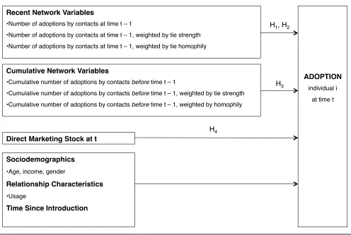
Figure 1 presents our conceptual model. The dependent variable is product adoption of individual i at time t. We include two main antecedents of adoption in the model: (1) network variables1 _{(recent adoptions, recent adoptions} weighted by tie strength and homophily, cumulative adop-tions, and cumulative adoptions weighted by tie strength and homophily) and (2) direct marketing stock. In addition, we control for sociodemographics and relationship charac-teristics (e.g., Arts, Frambach, and Bijmolt 2011; Prins and Verhoef 2007). To account for potential long-term effects of adoptions and direct marketing, we include stock measures with a carryover parameter for the cumulative adoptions and direct marketing. We include monthly dummies to account for the factors that affect all consumers in the mar-ket, such as the total number of adopters in the market and mass marketing by the firm. To account for potential time-varying effects, we allow the parameters of the social influ-ence variables and direct marketing to vary over time.

Dynamics of Social Influence

In line with previous studies, we examine the net effect of social influence in the context of successful product intro-ductions. That is, we focus on the impact of previous adop-tions on current adopadop-tions and find a positive effect on aver-age. Multiple studies in marketing have shown that the effects of marketing actions may vary over time and/or dur-ing the product life cycle (e.g., Leeflang et al. 2009; Osinga, Leeflang, and Wieringa 2010). Understanding of the effects of social influence over time on new product adoption is, however, limited.

1_{We thank an anonymous reviewer for suggesting this method}

In theorizing about this time-varying effect of social influence, scholars can take the perspective of either the adopter (influencer) or the potential adopter (person to be influenced). Taking the adopter’s perspective, there are two arguments for an adopter’s decreasing influence. First, early adopters are more contagious than later adopters because the former tend to score higher on new product involvement and opinion leadership (Rogers 2003; Van Eck, Jager, and Leeflang 2011). Consequently, they may exert a stronger influence on potential new adopters. Second, if the number of adopters has increased already, the marginal influence of a new adopter becomes smaller. This is in line with the non-uniform-influence diffusion models (Easingwood, Mahajan, and Muller 1983) and the contagion through Bayesian learning approach, as Roberts and Urban (1988) suggest. Both arguments posit that the effect of a recent additional adopter in one’s network on a potential adopter decreases over time, and neither argument automatically implies that the effect of cumulative adoptions decreases over time.

Taking the potential adopter’s perspective, a decreasing effect of social influence may occur because later adopters are less susceptible to social contagion than early adopters (Van den Bulte and Joshi 2007). In a two-segment setup, Van den Bulte and Joshi (2007) prove that having con-sumers vary in their sensitivity to contagion in a hazard model may result in a systematic decrease in the average

sensitivity to contagion as time goes by. This argument would imply a decreasing impact of all social influence variables.

In addition to the aforementioned two perspectives, the market perspective suggests a decreasing social influence over time. As time since introduction passes, knowledge about the product in the market increases. Moreover, the new product will have become the new standard in the mar-ket. Consequently, the importance of other information sources decreases. This so-called information substitution dynamic implies that the effect of recent adoptions among contacts would decrease over time (Chen, Wang, and Xie 2011), whereas the effect of cumulative adoptions is less clear. The cumulative number of adoptions signals to consumers what the norm has become in their network, leading to an increase over time of the effect of cumulative adoptions.

In summary, the aforementioned mechanisms tend to lessen the effect of recent adoptions among contacts on the adoption of an individual customer over time. However, the decreasing impact of the cumulative number of adoptions over time is less clear. An argument in support of this theory posits that potential adopters become less susceptible to contagion; however, the information substitution expla-nation suggests an increasing influence of contagion. There-fore, we only hypothesize a decreasing effect of recent adoptions and empirically explore a potential time-varying effect for the included cumulative adoption variables.

FIGURE 1 Conceptual Model

! ! ! ! !

ADOPTION!

individual i!

at time t!

Recent Network Variables!

•"Number of adoptions by contacts at time t – 1!

•"Number of adoptions by contacts at time t – 1, weighted by tie strength! •"Number of adoptions by contacts at time t – 1, weighted by tie homophily!

!

Sociodemographics!

•_"Age, income, gender!

Relationship Characteristics!

•"Usage!

Time Since Introduction!

Direct Marketing Stock at t!

!

H3!

H1, H2!

Cumulative Network Variables!

•"Cumulative number of adoptions by contacts before time t – 1!

•"Cumulative number of adoptions by contacts before time t – 1, weighted by tie strength! •"Cumulative number of adoptions by contacts before time t – 1, weighted by homophily!

H1: Smartphone adoptions that are (a) unweighted, (b)

weighted by tie strength, and (c) weighted by homophily in month t – 1 in an individual’s network positively affect the smartphone adoption probability of a customer in month t.

H₂: The effect of smartphone adoptions that are (a) unweighted, (b) weighted by tie strength, and (c) weighted by homophily in month t – 1 in an individual’s network on the smartphone adoption probability of a customer in month t decreases from the product introduction onward. H3: Cumulative smartphone adoptions that are (a) unweighted,

(b) weighted by tie strength, and (c) weighted by homophily in month t – 1 in an individual’s network positively affect the smartphone adoption probability of a customer in month t.

In addition to the time-varying effect of social influence (the period effect), the role of cumulative adoptions by other customers may show a decaying effect similar to other factors affecting consumer behavior (Hanssens, Par-sons, and Schultz 2001). As the time since adoption passes, the contagiousness of an adopter decreases, producing the so-called age effect (Du and Kamakura 2011; Kalish and Lilien 1986). The adopters’ tendency to talk about and show off their new product may decay because the novelty of the adoption decreases. Nitzan and Libai (2011) show a similar effect in a churn context. Thus, in our empirical assessment, we should account for decaying carryover effects in the cumulative social influence variables.

Direct Marketing

We define direct marketing as a personalized offer of a product (and/or service) that a customer does not yet own (Verhoef 2003). Van den Bulte and Lilien (2001) show that it is important to account for marketing effects when study-ing social influence on adoption decisions. Direct market-ing can create interest in a new product and may persuade consumers to purchase products by offering short-term rewards (Verhoef 2003). Several studies have shown that direct marketing affects customer behavior (e.g., in new product adoption; Hill, Provost, and Volinsky 2006; Prins and Verhoef 2007; Venkatesan and Kumar 2004). There-fore, we expect a positive effect of direct marketing on adoption.

Thus far, researchers in customer management have ignored time-varying effects of direct marking. In line with the theory of information substitution dynamics, we might expect that the effect of marketing decreases over time because marketing is an information source. Osinga, Leeflang, and Wieringa (2010) and Narayanan, Manchanda, and Chintagunta (2005), for example, show that the effect of detailing on sales of a new pharmaceutical drug decreases over time. However, direct marketing in a consumer prod-uct context is mostly persuasive. It is a call for action because it contains an offer or tailored information that is particularly relevant to the consumer (Godfrey, Seiders, and Voss 2011; Prins and Verhoef 2007). This call for action should provide the right information to the right customer at the right time, inducing adoption of the new product. Given the clear function of direct marketing as a persuasive behavior-focused instrument and given the adaptive nature

of the offer, we expect a positive effect of direct marketing that remains constant over time since the introduction of the new product. Thus, we hypothesize the following:

H_4a: Direct marketing positively affects a customer’s smart-phone adoption probability.

H_4b: The positive effect of direct marketing on a customer’s smartphone adoption probability is constant over time.

Data

Research Setting

We examine consumer adoption of an innovative product— namely, the smartphone, with either a physical keyboard or a touchscreen QWERTY keyboard, such as the Blackberry and the iPhone (Manes 2004). For our observation period, these mobile phones were considered innovative because they were fundamentally different from previous genera-tions of mobile phones. That is, they were developed for multimedia applications, online communication, and web browsing. Smartphones are high-technology products and are relatively expensive. Therefore, social interactions are likely to influence the adoption decision (Chen, Wang, and Xie 2011). We use individual data from a large, random sample of customers of a Dutch mobile telecommunications operator (n = 15,700).

Dependent Variable

The dependent variable is time of adoption, and we define it as the number of months between the telecommunications operator’s introduction of the smartphone (in April 2007) and a customer’s adoption of the product. We only include potential first-time adopters of a smartphone and thus omit customers with experience with the technology. During the observation period (April 2007–September 2009), 4,148 customers (26%) adopted a smartphone, so 74% ([(15,700 – 4,148)/ 15,700] ¥100) of the observations are censored. We included these censored observations in the estimation sam-ple to avoid problems with spurious duration dependence (Van den Bulte and Iyengar 2011). To illustrate the pattern of the adoptions over time, we provide the empirical hazard function in Figure 2. The empirical hazard in month t is the fraction of potential adopters adopting in month t. Adoption data are available only for customers and their contacts who

FIGURE 2

Empirical Hazard Function

2 4 6 8 10 12 14 16 18 20 22 24 26 28 .020

.015

.010

.005

.000

Month

H

a

za

are also customers of the company. The market share of the company was approximately 45% during this period, and thus the sample covers a substantial part of the market.

Explanatory Variables: Social Influence

We use CDRs of a mobile telecommunications operator to create networks. In CDR data, all phone calls and text mes-sages are included. We assume that the mobile phone network is a good proxy for a customer’s real social network and that it is constant over time (Haythornthwaite 2005). Prior research has used mobile call graphs to analyze network effects to model retention (Nitzan and Libai 2011) and adoption (Hill, Provost, and Volinsky 2006). The CDR data can easily be complemented with customer and relationship data because they come from a telecommunications operator that also has access to a corresponding customer database. Another advan-tage of calling data is that actual communications between consumers are observed, and thus, the strength of the rela-tionship can be inferred from the volume of communication. For this study, we collected CDR data during March, April, and May 2008. We only included phone calls and text messages to and from the telecommunications operator’s mobile phones made within the Netherlands. We used the CDR data to construct 15,700 ego networks, one for each customer in the sample. These networks consist of a focal person (ego) and all the people with whom he or she has a direct tie (alters). We define a tie as a reciprocal contact between two people through text messages and phone calls. We measure the strength of a tie as the ratio of the volume of communication over the tie to the total communication volume of the focal customer within the observation period of three months (Nitzan and Libai 2011; Onnela et al. 2007). For the communication, we take into account all within-country mobile telephony communication to and from all telecommunications operators. Thus, we account for the individual differences in communication volume and the degree centrality of a customer (i.e., the number of ties). Homophily, or “the principle that a contact between similar people occurs at a higher rate than among dissimilar people” (McPherson, Smith-Lovin, and Cook 2001, p. 416), is an important phenomenon in the analysis of social inter-actions. In line with previous work, we measure homophily on the basis of the similarity between customers on sociodemographic variables (Brown and Reingen 1987; Nitzan and Libai 2011). Specifically, we use four variables (age, gender, education level, and income), and similarity on each variable adds .25 to the homophily score (Brown and Reingen 1987; Nitzan and Libai 2011). We consider age similar if the difference is less than or equal to five years. The six variables we use to infer the effect of social influence in month t are the number of contacts that adopted in month t – 1 (NADOPTt – 1), the NADOPTt – 1variable weighted separately by tie strength and homophily, the cumulative number of adoptions among a customer’s con-tacts up to and including t – 2 (NADOPTSTOCKt – 2), and the NADOPTSTOCKt – 2variable also weighted separately by tie strength and homophily.

Next, it is difficult to assess whether the behavior of an individual in a group is caused by the group’s behavior or

whether the group’s behavior is caused by the behavior of the individual (Manski 2000). To avoid this so-called reflection problem, we included the number of adoptions by contacts as lagged variables. Finally, we use a carryover parameter (dADOPT) for the cumulative adoption variables with the same structure as the direct marketing stock variables (see the following subsection). To be consistent and parsimonious, we use the same carryover parameter for all cumulative adoption variables.

Explanatory Variables: Direct Marketing and Adopter Characteristics

An important aspect of modeling the effects of social influ-ence is ensuring that the effect can indeed be attributed to social interaction (Hartmann et al. 2008). Van den Bulte and Lilien (2001) find that the effects of social contagion disap-pear when marketing activities are taken into account. This is an example of correlated effects (Manski 2000): two people show similar behavior not because one influences the other but because both were influenced by a marketing campaign. Therefore, we include marketing efforts and monthly dummies in our model. We include marketing effort as a time-dependent explanatory variable based on monthly observations from April 2007 to September 2009. In particular, the time-dependent direct marketing variable is a stock variable indicating how many direct marketing actions (e-mail, text message, or bill supplement) a cus-tomer received. We only account for smartphone-related direct marketing actions. The focal company provided us with the direct marketing database, including a short description of each campaign, from which we selected only the relevant actions in close cooperation with the direct marketing expert of the firm. Following the market response modeling literature (Hanssens, Parsons, and Schultz 2001), we account for the possibility that direct marketing may have a longterm effect by including a carry -over parameter in our model. In particular, the direct mar-keting stock of individual i at time t (DMSTOCKit) is operationalized as DMSTOCKit = DMit + dDM ¥ DMSTOCKi, t – 1, in line with, for example, Iyengar, Van den Bulte, and Valente (2011).

the average monthly revenue that a customer generated over a one-year period (April 2007–March 2008). Firms frequently use these variables for target selection of direct marketing campaigns. By including these variables in our model, we also control for these effects beyond the Mund-lak approach (Prins and Verhoef 2007). Table 3 presents the operationalization of all variables.

Model Specification and Estimation

We use a fractional polynomial hazard model to analyze the time of adoption (Royston and Altman 1994; Sauerbrei, Royston, and Look 2007). The model is based on the stan-dard hazard model typically used to model time-to-event data (for applications in marketing, see Landsman and Givon 2010; Van den Bulte 2000). The hazard is the proba-bility that the event of interest will take place in the next period given that it did not yet occur. We use the comple-mentary log-log formulation of the hazard because the tim-ing of adoption is a continuous process that we analyze on a monthly interval basis (Allison 1982). As previously noted, we include monthly dummies to capture factors that affect all customers, such as mass-media advertising by the firm and the total number of adoptions in the market. Thus, we include monthly dummies to account for the changes in the likelihood of adoption over time, and we model the impact of having adopters in a network (i.e., social influence) across individuals within a period. Furthermore, including monthly dummies is the most flexible way to model the baseline hazard, which is increasing. The resulting discrete hazard model is commonly used for this type of problem (see Iyengar, Van den Bulte, and Valente 2011). We estimate the carryover parameters of the stock variables using a grid search before the estimation of the fractional polynomials because estimating all parameters simultaneously is infeasi-ble due to the size and complexity of the model.

Unobserved Heterogeneity

Unobserved heterogeneity, or frailty, is a well-known issue in duration models (Therneau and Grambsch 2000). We included a random intercept, the frailty term, in the model to account for omitted variables and the likely early adop-tion of those who are most frail (i.e., intrinsically most

likely to adopt). We included a Gaussian frailty term (ni~ N(0, W_n)) in the model.2

Accounting for Time-Varying Parameters

To incorporate time-varying parameters for social influence and direct marketing, we use a fractional polynomial approach (Berger, Schäfer, and Ulm 2003; Royston and Alt-man 1994).3 _{Lehr and Schemper (2007) show that this} method performs well. The fractional polynomial approach incorporates complex shapes of time-varying parameters. We use Berger, Schäfer, and Ulm’s (2003) suggested proce-dure to determine the optimal shape of the fractional poly-nomial. We define the time-varying parameter of variable X as bX, t= bX+ Smj=1(bXFPj¥t(pj)). We use a maximal degree of m = 2 and the set of powers P = {–2, –1, –.5, 0, .5, 1, 2, 3} (Berger, Schäfer, and Ulm 2003). For p = 0, we define bX, t= bX + bX, FP¥ ln(t), and for p1= p2= p, we define

bX, t = bX + bX, FP1 ¥ tp + bX, FP2 ¥ tp ¥ ln(t) (Berger, Schäfer, and Ulm 2003). We include time-varying parame-ters for social influence and direct marketing. We begin by estimating the polynomial structure for the variable with the lowest p-value in the base model (without the fractional polynomials). We determine the optimal values for the degree m and the powers pjby minimizing the p-values of the likelihood ratio tests in which we compare the model with and without the fractional polynomial. For these likeli-hood ratio tests, we use 2m degrees of freedom (Berger, Schäfer, and Ulm 2003). The likelihood ratio test is appro-priate here because it is a nested testing problem.

In addition to testing the significance of the time-varying effect compared with the constant effect, we examine whether adding the variable including the polynomials sig-nificantly improves model fit. For these tests, with 2m + 1 degrees of freedom, we apply a Bonferroni correction and multiply the p-values by 2 (Berger, Schäfer, and Ulm 2003).

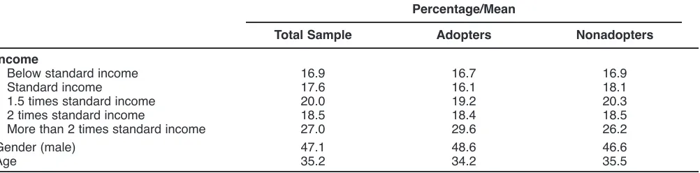
TABLE 2

Estimation Results of the Hazard Model of Adoption

Percentage/Mean

Total Sample Adopters Nonadopters

Income

Below standard income 16.9 16.7 16.9 Standard income 17.6 16.1 18.1 1.5 times standard income 20.0 19.2 20.3 2 times standard income 18.5 18.4 18.5 More than 2 times standard income 27.0 29.6 26.2 Gender (male) 47.1 48.6 46.6 Age 35.2 34.2 35.5

Notes: Due to confidentiality issues, we do not show the descriptives of the usage variable.

2_{We also specified a model with random effects for contagion.}

Unfortunately, we were not able to estimate this model with random effects of the social influence variables. The estimation procedure did not converge, and therefore, we did not obtain reliable output.

3_{We use an established estimation procedure, which consists of}

Variable Operationalization Formula

D₂, ..., D₂₈ Dummy variables indicating the month of the observation period Tie A reciprocal contact between two people i and j: i should have

contacted j at least once (i Æj), and j should have contacted i at least once (j Æi) by a call or a text message

NCALLS_ij Number of calling minutes over tie i–j during the three-month network observation period

NTEXTS_ij Number of text messages over tie i–j during the three-month network observation period

Communication volume (CV_ij)

The sum of the number of calling minutes and the number of text messages during the three-month observation period for tie i–j

NCALLS_ij+ NTEXTS_ij

Total communication volume (TCV_i)

The sum of the communication volume for all ties of a focal cus-tomer i within and outside the telecommunications operator’s network (ego network total, ENT_i)

CV_ij

j ENTi

∑

∈

Tie strength (TS_ij) The ratio of the volume of communication of tie i–j to the total communication volume of focal customer i within the network observation period of three months

CV TCV

ij

i

Homophily (HOM_ij) The similarity between customers i and j in age, gender, educa-tion level, and income. Similarity on each variable adds .25 to the homophily score. Age is considered similar if the difference is less than or equal to five years.

Adoption (AD_jt) A binary variable indicating whether contact j adopted in month t (1 = yes, 0 = no)

NADOPT_{t – 1} The number of contacts in the ego network of the focal cus-tomer i on the telecommunications operator network (ego net-work, EN_i) who adopted in month t – 1

ADj, t 1 j ENi

∑

−

∈

NADOPTSTOCK_{t – 2} The cumulative adoptions up to and including t – 2, using a car-ryover parameter (dADOPT)

NADOPTi, t – 2+ dADOPT

¥NADOPTSTOCKi, t – 3

NADOPTSTR_{t – 1} Number of adopters in the ego network of the focal customer in

month t – 1 weighted by tie strength TSij ADj, t 1

j ENi

∑

× ₋

∈

NADOPTSTRSTOCK_{t – 2} Stock variable of NADOPTSTR up to and including t – 2 NADOPTSTRi, t – 2+ dADOPT

¥NADOPTSTRSTOCKi, t – 3

NADOPTHOM_{t – 1} Number of adopters in the ego network of the focal customer in

month t – 1 weighted by homophily HOMij ADj, t 1

j ENi

∑

× −

∈

NADOPTHOMSTOCK_{t – 2} Stock variable of NADOPTHOM up to and including t – 2 NADOPTHOMi, t – 2+ dADOPT

¥NADOPTHOMSTOCKi, t – 3

DMAVG_t Percentage of weeks in which a direct marketing was received

during the observation period DM

T it 0 T

i i

∑

DMSTOCKt Stock variable of direct marketing up to and including t DMi, t – 1+ dDM

¥DMSTOCK_{i, t – 2}

AGE Age (in years)

USAGE Natural logarithm of the average monthly revenue (euros) over a one-year period

INCOME 1 = below standard income, 2 = standard income, 3 = 1.5 ¥

standard income, 4 = 2 ¥standard income, 5 [reference category] = more than 2 ¥standard income

GENDER Gender dummy (0 [reference category] = female, 1 = male) FPY_VARIABLE Variable used to estimate the parameter of fractional polynomial

Y (Y = 1, 2) of variable “VARIABLE” TABLE 3

4_{The results are available from the first author upon request.} 5_{To assess the out-of-sample performance of our final model,}

we use the first 28 months for model estimation and use the lift approach that Katona, Zubcsek, and Sarvary (2011) suggest to assess the predictive validity. The full model with time-varying parameters has a higher lift (1.841) than the basic model without time-varying parameters (1.699). Because the main goal of this study is to determine and describe the time-varying effects, we focus on the in-sample model selection and results.

In the model, we define the hazard of adoption of customer i in month t as a function of explanatory variables (for an explanation of the labels, see Table 3):

We used the package glmmML in R version 2.15.1 (Broström and Holmberg 2011) to fit a generalized linear model with random intercepts using maximum likelihood and numerical integration using Gauss–Hermite quadrature.

Results

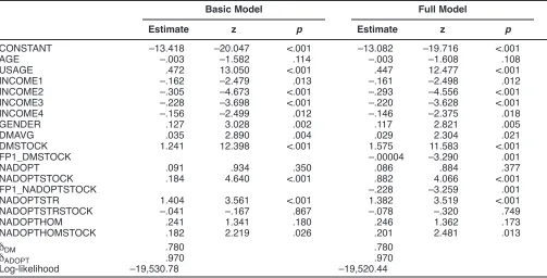
The left-hand columns in Table 4 show the parameter esti-mates of the basic model (i.e., the model without time-varying effects). We highlight three important findings from the basic model. First, we used this model to find the optimal values for the carryover parameters by means of a grid search. The carryover parameter of the direct marketing stock (dDM) is .78, which is in the range of values from ear-lier research (Leone 1995). The carryover parameter for the cumulative adoption variables (dADOPT) is equal to .97. This implies that the contribution of each adoption in a cus-tomer’s ego network to the social influence effect decreases

[

(

)

]

slowly from the adoption moment onward. Second, we find that the parameter of DMAVG, which we included to account for endogeneity by means of the Mundlak (1978) approach, is significantly positive (b36 = .035, p= .004). This parameter captures the effect that customers who receive more direct marketing are more likely to adopt in the first place. Finally, three of the six parameters of the social influence variables are positive and significant. The effects of the number of (1) recent adoptions, (2) recent adoptions weighted by homophily, and (3) cumulative adoptions weighted by tie strength are not significant, but because we theoretically argued that all operationalizations of social influence are important, we keep the variables in the model and subsequently investigate potential time-varying effects.

Hypothesis Testing

We use the p-values of the parameters in the basic model to determine the order of estimating the fractional polynomials for the marketing stock and the four social influence variables. In order from smallest to largest p-value, the variables are DMSTOCK, NADOPTSTOCK, NADOPTSTR, NADOPTHOMSTOCK, NADOPTHOM, NADOPT, and NADOPTSTRSTOCK. We estimated models for all possible combinations of powers with degrees 1 and 2. Table 5 shows the results of the tests in the fractional polynomial procedure. For the DMSTOCK variable, one polynomial with power 3 leads to the largest improvement in model fit (log-likelihood = –19,525.47, p< .01). Next, we determined the optimal poly-nomial for the parameter of the NADOPTSTOCK variable. The optimal model, based on the p-values of the likelihood ratio tests, had degree 1 and power 0 (log-likelihood = –19,520.44, p < .01). For the other five social influence variables, adding fractional polynomials did not significantly improve the model fit.4_{We present the parameter estimates} of this model (the full model) in the right-hand columns of Table 4. We next discuss the results in more detail.5

Among the recent adoption variables, only the parame-ter of the recent adoptions weighted by tie strength is posi-tive and significant (b40 = 1.382, p< .001). Furthermore, this effect is constant over time. These findings support H1b but do not support H1a, H1c, H2a, H2b, or H2c. Among the cumulative adoption variables, the parameter of the cumu-lative number of adoptions is positive and significant and varies over time (b39 = .882, p< .001; b39¢ = –.228, p =

.001). Figure 3, Panel A, shows the time-varying effect of this variable, which is calculated as b39,t= b39+ b39¢¥ln(t).

of the cumulative number of adoptions weighted by homophily is also positive and significant but does not vary over time (b43= .201, p= .013). These results provide sup-port for H3c. The effect of the cumulative number of adop-tions weighted by tie strength is not significant, and thus, H3b is not supported. Figure 3, Panel B shows the time-varying effect of the direct marketing stock, which is b37, t=

b37 + b37¢¥t3. The effect is positive and significant in all

periods but decreases from a value of 1.58 in month 1 to approximately .61 in month 28. These findings support H4a but do not support H4b.

In line with prior research, we find significant effects of income, gender, and service usage. Income is positively related to adoption; higher income groups (two times the standard income and higher) are more likely to adopt than lower-income groups (all p-values < .05). Men are more likely to adopt than women (p= .005). Finally, we find that customers with high service usage levels are more inclined to adopt as well (p< .001; see also Prins and Verhoef 2007).

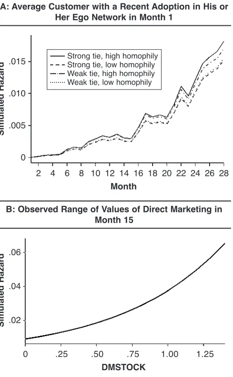
Simulation Results

We use the parameter estimates of the full model to simulate the hazard of adoption for an average customer to facilitate interpretation of our findings. To illustrate the effect of an adoption in the ego network of the average customer in the first month after the product introduction, we simulate four scenarios on the basis of the type of contact: tie strength (weak, strong) ¥homophily (high, low). With this simulation, we can analyze the impact of an adoption of different types of contacts over the entire observation period. Figure 4, Panel A, presents the results. It shows that the hazard is largest when a contact who is similar (high homophily) and socially close (strong tie) adopted. Furthermore, the difference in the hazard between the high and low homophily scenarios is larger than between the strong and weak tie scenarios.

In addition to the simulations, we assess the importance of the network characteristics homophily and tie strength by applying a leave-one-out approach. We compare the model fit of the full model with (1) the fit of the full model without

TABLE 4

Estimation Results of the Hazard Model of Adoption

Basic Model Full Model

Estimate z p Estimate z p

CONSTANT –13.418 –20.047 <.001 –13.082 –19.716 <.001

AGE –.003 –1.582 .114 –.003 –1.608 .108

USAGE .472 13.050 <.001 .447 12.477 <.001 INCOME1 –.162 –2.479 .013 –.161 –2.498 .012

INCOME2 –.305 –4.673 <.001 –.293 –4.556 <.001 INCOME3 –.228 –3.698 <.001 –.220 –3.628 <.001 INCOME4 –.156 –2.499 .012 –.146 –2.375 .018

GENDER .127 3.028 .002 .117 2.821 .005

DMAVG .035 2.890 .004 .029 2.304 .021

DMSTOCK 1.241 12.398 <.001 1.575 11.583 <.001 FP1_DMSTOCK –.00004 –3.290 .001

NADOPT .091 .934 .350 .086 .884 .377

NADOPTSTOCK .184 4.640 <.001 .882 4.066 <.001 FP1_NADOPTSTOCK –.228 –3.259 .001

NADOPTSTR 1.404 3.561 <.001 1.382 3.519 <.001 NADOPTSTRSTOCK –.041 –.167 .867 –.078 –.320 .749

NADOPTHOM .241 1.341 .180 .246 1.362 .173

NADOPTHOMSTOCK .182 2.219 .026 .201 2.481 .013

dDM .780 .780

dADOPT .970 .970

Log-likelihood –19,530.78 –19,520.44

Notes: We omitted the monthly dummies from the table for clarity.

TABLE 5

Model Comparison Results

LR Test for Adding LR Test for Adding Model Description Log-Likelihood the Polynomial the Variablea

1 Basic model without DMSTOCK –19,599.25 2 Basic model –19,530.78

3 Basic model + DMSTOCK (m = 1, p= 3) –19,525.47 c2_{(d.f. = 2) = 10.63, c}2_{(d.f. = 3) = 147.57,}

p< .01 pb_{< .01}

4 Model 3 without NADOPTSTOCK –19,535.67

5 Full model: Model 3 with –19,520.44 c2_{(d.f. = 2) = 10.05, c}2_{(d.f. = 3) = 30.46,}

NADOPTSTOCK (m = 1, p= 0) p< .01 pb_{< .01}

a_{Includes the polynomial.}

the homophily-weighted adoptions, (2) the full model with-out the strength-weighted adoptions, and (3) the full model without the homophily- and strength-weighted adoptions. Model fit decreases in all cases, and the decrease achieved by deleting the homophily- or strength-weighted adoptions is in the same order of magnitude (–3.42 and –5.15), in which the decrease of deleting the strength-weighted adop-tions is slightly larger. Deleting these adopadop-tions leads to a change in model fit of –9.17.

To illustrate the nonlinear effect of direct marketing, we simulated the hazard for an average customer in the middle of the observation period in Month 15. We use the observed range of values for the direct marketing variable. Figure 4, Panel B, shows the result of this simulation. The line is increasingly upward sloping. The hazard of adoption of an average customer with a high DMSTOCK (hazard = .07) is approximately seven times higher than the hazard of an average customer with no DMSTOCK.

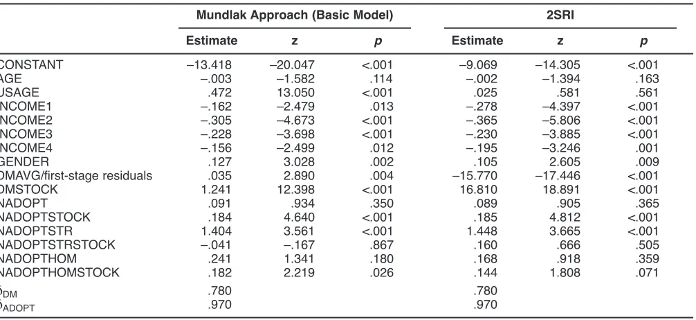
Robustness Checks

We use the Mundlak approach (Mundlak 1978; Verbeek 2008, p. 156) to account for potential endogeneity caused by the possibility that the company is more likely to target likely adopters. To investigate the robustness of our find-ings, we reestimated the basic model (without the time-varying effects) using a different approach to deal with

potential endogeneity, namely, two-stage residual inclusion (2SRI; Terza, Basu, and Rathouz 2008). Two-stage residual inclusion is similar to two-stage least squares (2SLS), a commonly used instrumental variable approach for linear regression models (see, e.g., Greene 2012, p. 270). How-ever, for nonlinear models, the 2SLS estimator is not con-sistent, whereas the 2SRI estimator is (Terza, Basu, and Rathouz 2008). The difference between 2SRI and 2SLS occurs in the second stage. In the second stage of 2SRI, the first-stage residuals are added to the main equation, imply-ing that both the endogenous regressor and the first-stage residuals are included, whereas in the second stage of 2SLS, the endogenous regressor is replaced by the fitted values of the first stage. We used the variable “months remaining in the current contract” (as dummies) as the instrument.6_{This is a set of 12 dummy variables indicating} whether a customer has 0, 1, 2, ..., 11 months left in his or her current contract in month t. We assumed that all con-tracts would end within 12 months because we did not have detailed information on the type of contract. However, most 2 4 6 8 10 12 14 16 18 20 22 24 26 28

1.2

1.0

.8

.6

.4

.2

0

Month

Effe

c

t

2 4 6 8 10 12 14 16 18 20 22 24 26 28 1.8

1.6 1.4 1.2 1.0 .8 .6 .4 .2

Month

Effe

c

t

±2 SE Mean

±2 SE Mean

FIGURE 3 Time-Varying Effects

A: Cumulative Unweighted Adoptions (NADOPTSTOCK)

B: Direct Marketing (DMSTOCK) 2 4 6 8 10 12 14 16 18 20 22 24 26 28

.015

.010

.005

0

Month

Si

m

u

la

te

d

H

a

za

rd

.25 .50 .75 1.00 1.25

0 .06

.04

.02

DMSTOCK

Si

m

u

la

te

d

H

a

za

rd

Strong tie, high homophily Strong tie, low homophily Weak tie, high homophily Weak tie, low homophily

FIGURE 4 Simulated Hazards

A: Average Customer with a Recent Adoption in His or Her Ego Network in Month 1

B: Observed Range of Values of Direct Marketing in Month 15

contracts were one-year contracts, and all contracts were automatically prolonged by one year at that time. We find that the results of the two models do not differ substantively (see Table 6). Given the similarity of the results of the Mundlak approach and 2SRI, as well as the complexity resulting from the 2SRI approach (i.e., adding another time-dependent covariate to the model), we use the model specifi-cation including the Mundlak variable for the full model.

In the years since the introduction of the smartphone, the smartphone market has become more mature. There-fore, churners from the focal company may actually be adopters of a smartphone at a competing firm. However, we do not have data on where customers go and what they do after churning from the focal company. To investigate to what extent our results are affected by this phenomenon, we reestimated the full model by treating churners as adopters.7 As we expected, the effects of some of the control variables change because churn and adoption effects are partly mixed up in this model. Therefore, we should carefully interpret the outcomes of this analysis. Most importantly, though, our key findings are robust to this extreme check.

To assess the stability of our model results, we validated our model on ten samples consisting of 80% of the original data (Bolton, Lemon, and Verhoef 2008). The parameter estimates are stable across the ten samples, and the substan-tive findings hold in each sample.8_{In summary, the checks} illustrate that our key findings are robust against different model specifications and variable operationalizations.

Discussion

During the past decade, marketers have shown a renewed interest in the effects of social influence on customer

behav-ior. Social network data are becoming easier to obtain, and firms are searching for ways to compensate for the decreas-ing effectiveness of traditional instruments, such as mass-media advertising. This study investigates the dynamic social influence effects of recent and cumulative adoptions in a customer’s network on his or her adoption, accounting for direct marketing efforts of the firm. Table 7 shows a summary of the hypotheses testing. Our study presents the following key findings:

•Social influence affects adoption through different social influence variables, even when we account for direct market-ing effects. This provides additional evidence for Godes’s (2011) claim that social influence effects are now well estab-lished. However, our findings also indicate that the effects of social influence are more complex than generally assumed. •Tie strength and homophily are both important as weighting

factors in models of social influence.

•Recent adoptions in a customer’s ego network remain equally influential from the production introduction onward. •The effect of the cumulative adoptions in a customer’s ego

network is positive and decreases from the product introduc-tion onward.

•The effect of direct marketing is positive, but it also decreases from the product introduction onward.

These findings have several implications for marketing theory, and specifically social network theory within mar-keting. The constant impact of recent adoptions contradicts our initial hypotheses, which are based on existing theory. This constant impact has three possible implications. First, it suggests that adopters remain equally contagious from the product introduction onward. In other words, adopters are enthusiastic and share their opinion with their social net-work immediately after the adoption, regardless of when the adoption occurs. Second, it also suggests that each addi-tional adopter has an influence and that this influence does not become smaller, as the diffusion literature has suggested (Easingwood, Mahajan, and Muller 1983; Roberts and 7_{The results are available upon request from the first author.}

8_{We omitted the table with estimation results because of its size.}

The results are available upon request from the first author.

TABLE 6

Comparison of Parameter Estimates Using the Mundlak Approach and 2SRI

Mundlak Approach (Basic Model) 2SRI

Estimate z p Estimate z p

CONSTANT –13.418 –20.047 <.001 –9.069 –14.305 <.001

AGE –.003 –1.582 .114 –.002 –1.394 .163

USAGE .472 13.050 <.001 .025 .581 .561

INCOME1 –.162 –2.479 .013 –.278 –4.397 <.001 INCOME2 –.305 –4.673 <.001 –.365 –5.806 <.001 INCOME3 –.228 –3.698 <.001 –.230 –3.885 <.001 INCOME4 –.156 –2.499 .012 –.195 –3.246 .001

GENDER .127 3.028 .002 .105 2.605 .009

DMAVG/first-stage residuals .035 2.890 .004 –15.770 –17.446 <.001 DMSTOCK 1.241 12.398 <.001 16.810 18.891 <.001 NADOPT .091 .934 .350 .089 .905 .365

NADOPTSTOCK .184 4.640 <.001 .185 4.812 <.001 NADOPTSTR 1.404 3.561 <.001 1.448 3.665 <.001 NADOPTSTRSTOCK –.041 –.167 .867 .160 .666 .505

NADOPTHOM .241 1.341 .180 .168 .918 .359

NADOPTHOMSTOCK .182 2.219 .026 .144 1.808 .071

dDM .780 .780

Urban 1988). Third, consumers remain equally affected by this behavior. This implication contrasts with the findings of Iyengar, Van den Bulte, and Valente (2011), who show that self-reported opinion leaders adopt earlier and are less susceptible to social influence. If susceptibility indeed increases from the product introduction onward, our results imply that this increase in susceptibility is compensated by a decrease in contagiousness, resulting in the constant effect we find. We are not able to disentangle these two factors in the current study.

Importantly, although we did not find evidence for a time-varying effect of recent adoptions, we did provide evi-dence for a period effect of the cumulative adoptions. The behavior of the ego network as a whole becomes less conta-gious, or consumers become less susceptible to its influence. In other words, the impact of local social pressure decreases from the product introduction onward. This decreasing effect is in line with both recent work on social influence on adoption (Bell and Song 2007; Choi, Hui, and Bell 2010) and the diffusion literature (Easingwood, Mahajan, and Muller 1983; Van den Bulte and Lilien 1997). Our findings thus show that the decrease of the imitation parameter q in the Bass model (Van den Bulte and Lilien 1997) may be due to a genuine decrease in the effect of social influence of the total number of adopters and not to the decreasing social influence of recent adopters. Furthermore, our results also show that the decrease in q over time is not caused by the length of the estimation period or the estimation procedure, as Van den Bulte and Stremersch (2004) show.

We provide evidence for age effects of social influence, in that the carryover parameter of the cumulative adoptions is .97; the contribution of each adoption in a customer’s ego

net-work to the social influence effect decreases slightly from the adoption moment onward. Most studies ignore these age effects and simply use the cumulative adoptions (see Table 1). We are among the first to empirically assess this age effect. In the area of social networks in marketing, two metrics have been extensively discussed: tie strength and homophily (Van den Bulte and Wuyts 2007). Our fine-grained analysis of social influence on adoption reveals that tie strength and homophily are both important as weighting factors in models of social influence. In addition to the unweighted adoptions, the weighted variables significantly improve model fit, but each has a different effect. The recent adoptions weighted by tie strength and the cumula-tive adoptions weighted by homophily significantly affect adoption. A potential explanation for this difference is that strong ties are most persuasive shortly after adopting a product, whereas in the long run, the norm in a person’s net-work is set by homophilous others.

The results show an age effect of direct marketing: a direct marketing action contributes to the marketing stock for multiple periods but in a decreasing manner. Further-more, there is a period effect, meaning that the effect of the direct marketing stock variable decreases from the product introduction onward. Although we expected the direct mar-keting effect to be constant in the consumer context we studied, the decreasing effect is in line with previous research in other settings (Narayanan, Manchanda, and Chintagunta 2005; Osinga, Leeflang, and Wieringa 2010). This suggests that either direct marketing becomes less per-suasive from the product introduction onward or that, simi-lar to the role of detailing, the informative effect decreases (Narayanan, Manchanda, and Chintagunta 2005).

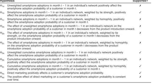
TABLE 7

Summary of the Hypothesis-Testing Results

Hypothesis Supported?

H_1a Unweighted smartphone adoptions in month t – 1 in an individual’s network positively affect the ✗

smartphone adoption probability of a customer in month t.

H1b Smartphone adoptions in month t – 1 in an individual’s network, weighted by tie strength, positively ✓

affect the smartphone adoption probability of a customer in month t.

H_1c Smartphone adoptions in month t – 1 in an individual’s network, weighted by homophily, positively ✗

affect the smartphone adoption probability of a customer in month t.

H2a The effect of unweighted smartphone adoptions in month t – 1 in an individual’s network on the ✗

smartphone adoption probability of a customer in month t decreases from the product introduction onward. H_2b The effect of smartphone adoptions in month t – 1 in an individual’s network, weighted by tie ✗

strength, on the smartphone adoption probability of a customer in month t decreases from the product introduction onward.

H2c The effect of smartphone adoptions in month t – 1 in an individual’s network, weighted by homophily, ✗

on the smartphone adoption probability of a customer in month t decreases from the product introduction onward.

H_3a Unweighted cumulative smartphone adoptions in month t – 1 in an individual’s network positively ✓

affect the smartphone adoption probability of a customer in month t.

H3b Cumulative smartphone adoptions in month t – 1 in an individual’s network, weighted by tie strength, ✗

positively affect the smartphone adoption probability of a customer in month t.

H_3c Cumulative smartphone adoptions in month t – 1 in an individual’s network, weighted by homophily, ✓

positively affect the smartphone adoption probability of a customer in month t.

H4a Direct marketing positively affects a customer’s smartphone adoption probability. ✓

H_4b The positive effect of direct marketing on a customer’s smartphone adoption probability is constant ✗