Database-Driven Real-Time Heuristic Search
in Video-Game Path
fi
nding
Ramon Lawrence
, Member, IEEE
, and Vadim Bulitko
Abstract—Real-time heuristic search algorithms satisfy a con-stant bound on the amount of planning per action, independent of the problem size. These algorithms are useful when the amount of time or memory resources are limited, or a rapid response time is required. An example of such a problem is pathfinding in video games where numerous units may be simultaneously required to react promptly to a player’s commands. Classic real-time heuristic search algorithms cannot be deployed due to their obvious state revisitation (“scrubbing”). Recent algorithms have improved per-formance by using a database of precomputed subgoals. However, a common issue is that the precomputation time can be large, and there is no guarantee that the precomputed data adequately cover the search space. In this paper, we present a new approach that guarantees coverage by abstracting the search space, using the same algorithm that performs the real-time search. It reduces the precomputation time via the use of dynamic programming. The new approach eliminates the learning component and the resultant “scrubbing.” Experimental results on maps of tens of millions of grid cells fromCounter-Strike: Sourceand benchmark maps from
Dragon Age: Origins show significantly faster execution times and improved optimality results compared to previous real-time algorithms.
Index Terms—Database, game pathfinding, real-time search.
I. INTRODUCTION
A
S search problems become larger, the amount of memory and time to produce an optimal answer using standard search algorithms, such as A [1], tend to increase substantially. This is an issue in resource-limited domains such as video-game pathfinding. In real-time search, the amount of planning time per move is bounded independently of the problem size.1This is useful when an agent does not have time to compute the entire plan before making a move.Classic heuristic algorithms, such as learning real-time A (LRTA ) [2], satisfy the real-time operation constraint via learning and consequently tend to repeatedly visit (“scrub”) the
Manuscript received May 11, 2012; revised July 06, 2012; accepted November 25, 2012. Date of publication November 29, 2012; date of current version September 11, 2013. This work was supported by the National Science and Engineering Research Council.
R. Lawrence is with the Department of Computer Science, University of British Columbia Okanagan, Kelowna, BC V1V 1V7 Canada (e-mail: ramon. [email protected]).
V. Bulitko is with the Department of Computing Science, University of Al-berta, Edmonton, AB T6G 2E8 Canada (e-mail: [email protected]).
Color versions of one or more of thefigures in this paper are available online at http://ieeexplore.ieee.org.
Digital Object Identifier 10.1109/TCIAIG.2012.2230632
1More precisely, of the number of states.
same states. Not only does such behavior yield poor solution quality, but it also appears irrational, which has prevented deployment of such algorithms in video games. Extensions to LRTA , such as LSS LRTA [3], improve solution quality but still allow an agent to revisit a state multiple times.
The performance of real-time search algorithms can be im-proved by using an offline precomputation stage that provides additional information to guide the search online. Algorithms such as D LRTA [4] and kNN LRTA [5] use precomputed subgoal databases to deal with inaccuracies in the heuristic function, thereby reducing the amount of learning and the resulting “scrubbing.” However, as the search space grows, the database precomputation time becomes prohibitively long in practice. Additionally, the solution quality varies substantially as the database coverage and quality are uneven throughout the space. LRTA with subgoals [6] computes subgoals to escape heuristic depressions and stores them as a tree of subgoals for each state. This provides more complete coverage, but still requires considerable space and time for the precomputation.
The contribution of this paper is a new retime search al-gorithm called hill-climbing and dynamic programming search (HCDPS) that outperforms previous state-of-the-art algorithms by requiring less precomputation time, having faster execution times, and virtually eliminating state revisitation. This contribu-tion is achieved via two ideas. First, instead of using a generic way of partitioning the map, such as into cliques [7] or sectors [8], we partition the map into reachability regions. The reacha-bility is defined with respect to the underlying pathfinding algo-rithm, which guarantees that the agent can traverse such regions without any state revisitation or learning. This allows us to re-place a learning algorithm (e.g., LRTA ) with simple greedy hill climbing. Doing so simplifies the algorithm, virtually eliminates scrubbing, and reduces the agent’s online memory footprint.
The second idea is applying dynamic programming to data-base precomputation. Once we partition the map into regions of hill-climbing reachability, we use dynamic programming in the region space to approximate optimal paths between representa-tives of any two such regions. This is in contrast to computing optimal paths for all region pairs with A , as done in D LRTA [4] or, by computing subgoals for every start/goal state combi-nation, as done in LRTA with subgoals [6]. In our experiments, the benefit of this approximation is a two orders of magnitude speedup in the database precomputation time.
Together, these two ideas, applied in the domain of pathfinding on video game maps of over ten million states, enable HCDPS to take less than 2 min of precomputation per map, have a path suboptimality of about 3%, per-move plan-ning time of 1 s, and an overall planning time two orders of
magnitude lower than A . HCDPS has substantially improved precomputation time and suboptimality compared to D LRTA , kNN LRTA , and LRTA with subgoals. When applied to benchmarking maps from Dragon Age: Origins, HCDPS had similar runtime performance but with map precomputation of between 5 and 30 s.
The organization of this paper is as follows. In Section II, we formulate and define the pathfinding heuristic search problem studied in this work. Section III covers related work on real-time and non-real-time heuristic search algorithms. An overview of the approach is given in Section IV, and Section V covers extensive details on the implementation and optimization of the algorithm. Different algorithm variations are explained in Section VI, and a theoretical analysis follows in Section VII. Experimental results are in Section VIII, and the paper closes with future work and conclusions.
II. PROBLEMFORMULATION
We define a heuristic search problem as a directed graph con-taining afinite set of states and weighted edges and two states designated as start and goal. At every time step, a search agent has a single current state, a vertex in the search graph, which it can change by taking an action (i.e., traversing an edge out of the current state). Each edge has a positive cost associated with it. The total cost of edges traversed by an agent from its start state until it arrives at the goal state is called the solution cost. We re-quire algorithms to be complete (i.e., produce a path from start to goal in afinite amount of time if such a path exists). Accord-ingly, we adopt the standard assumption of safe explorability of the search space and assume that the goal state can be reached from any state reachable from the start state.
An agent plans its next action by considering states in a local search space surrounding its current position. A heuristic func-tion (or simply heuristic) estimates the optimal travel cost be-tween a state and the goal. It is used by the agent to rank avail-able actions and select the most promising one. We require that the heuristic be available for any pair of states. We consider only admissible and consistent heuristic functions, which do not overestimate the actual remaining cost to the goal and whose difference in values for any two states does not exceed the cost of an optimal path between these states. This is required for our complexity results that involve A .
In real-time heuristic search, the amount of planning the agent does per action has an upper bound that does not depend on the total number of states in the problem space. We measure the move time as the mean planning per action in terms of cen-tral processing unit (CPU) time. Hard cutoffs of planning time are enforced by ensuring that the maximum move time for any move is below a given limit. The second key performance mea-sure of our study is suboptimality, defined as the ratio of the so-lution cost found by the agent to the optimal soso-lution cost minus one and times 100%. To illustrate, suboptimality of 0% indicates an optimal path and suboptimality of 50% indicates a path 1.5 times as costly as the optimal path.
In principle, all algorithms in this paper are applicable to any heuristic search problem as defined above. However, algorithms based on precomputation are best suited for problems where the search space can be efficiently enumerated. Search algorithms
that do not perform precomputation are also practically bounded by the constraint of storing heuristic values for each state vis-ited in the search space. Representing heuristic values for a large search space may not be practical. Finally, all algorithms are evaluated assuming that the state space is static. When a state space changes on thefly, precomputation algorithms are af-fected as the precomputation may be invalidated due to changes. In addition, algorithms based on LRTA are negatively affected by state–space changes during their operation as heuristics may not be correct. Handling state–space changes is out of the scope of this paper.
The presentation and experimental focus for this paper is pathfinding on grid-based video-game maps. States are vacant square grid cells. Each cell is connected to four cardinally (i.e., N, E, W, S) and four diagonally neighboring cells. Edges out of a vertex are moves available in the corresponding cell, and we will use the terms “action” and “move” interchangeably. Edges in the cardinal direction have a cost of 1, while diagonal edges cost 1.4. Throughout the paper, we use octile distance as our heuristic. It is thede factostandard heuristic in grid maps with diagonal edges and is defined as
where and are ab-solute values of the differences in - and -coordinates of the two states between which the heuristic distance is computed. In the absence of occupied grid cells, the octile distance gives the true shortest distance between any two states.
III. RELATEDWORK
Heuristic search algorithms can be classified as either real-time or non-real-real-time. A real-real-time heuristic search algorithm guarantees a constant bound on planning time per action. Algo-rithms such as A , IDA [9], and minimal-memory abstraction [8] are non-real-time, as they produce a complete (possibly ab-stract) solution before thefirst action is taken. As the problem size increases, the planning time and corresponding response time will exceed any set limit. The primary focus of this paper is on real-time search algorithms, but we also compare some non-real-time heuristic search algorithms.
A. Real-Time Heuristic Search Algorithms
Real-time search algorithms repeatedly interleave planning (i.e., selecting the most promising action) and execution (i.e., performing the selected action). This allows actions to be taken without solving the entire problem, which improves response time at the potential cost of suboptimal solutions. As only a par-tial solution exists when it is time to act, the selected action may be suboptimal (e.g., lead the agent into a corner). To improve the solution over time, most real-time search algorithms up-date/learn their heuristic. The learning process frequently causes the agent to “scrub” (i.e., repeatedly revisit) states to fill in heuristic local minima or heuristic depressions [10]. This de-grades solution quality and makes the algorithm unusable for video-game pathfinding.
the local search space in order to speed up learning. This signif-icantly improves suboptimality and the number of state revisits but does not eliminate the scrubbing problem and can still result in highly suboptimal paths.
Significant performance improvement is possible by solving a number of problems offline and storing them in a database. Then, online, these solved problems can be used to guide the agent by directing it to a nearby subgoal instead of a distant goal. Most heuristic functions are more accurate around their goal state. This is because heuristic functions are usually de-rived by ignoring certain intricacies of the search space (e.g., the octile distance heuristic ignores obstacles), and, thus, the closer to the goal, the fewer intricacies/obstacles are ignored and the more accurate the heuristic becomes. Hence, by following a se-quence of nearby subgoals, the agent benefits from a more ac-curate heuristic and, thus, has to do less learning.
There are several, previously developed, real-time heuristic search algorithms that use precomputed subgoals. D LRTA ab-stracts the search problem using the clique abstraction of PRA [7] and then builds a database of optimal paths between all pairs of ground-level representatives of distinct abstract states. The database does not store the entire path but only the ground-level state where the path enters the next region. Online, the agent repeatedly queries the database to identify its next subgoal and runs LRTA to it. The issues with D LRTA are the large amount of memory used and the lengthy precomputation time. Further, D LRTA repeatedly applies the clique abstraction, thereby cre-ating large irregular regions. As a result, the abstract regions can contain local heuristic depressions, thereby trapping the under-lying LRTA agent and causing learning and scrubbing.
kNN LRTA attempts to address D LRTA ’s shortcomings by not using a state abstraction and instead precomputing a given number of optimal paths between randomly selected pairs of states. Each optimal path is compressed into a series of states, such that each of them can be hill climbed to from the previous one. Online, a kNN LRTA agent uses its database in an attempt tofind a similar precomputed path and then runs LRTA to the associated subgoal. kNN LRTA ’s random database records do not guarantee that a suitable precomputed path will be found for a given problem. In such cases, kNN LRTA runs LRTA to the global goal, which subjects it to heuristic depressions and leads to learning and scrubbing. Additionally, precomputing D LRTA and kNN LRTA databases can be time consuming (e.g., over 100 h for a single video-game map).
LRTA with subgoals [6] precomputes a subgoal tree from each goal state where a subgoal is the next target state to exit a heuristic depression. Online, LRTA will be able to use them to escape a heuristic depression. However, the algorithm has no way of preventing scrubbing when it tries to reach the closest subgoal in the tree. Another issue is that the number of subgoals is large as there is a subgoal tree for each goal state, and the precomputation time is long.
TBA [11] is not based on LRTA and runs a time-sliced version of A instead. It does not use subgoals and always computes its heuristic with respect to the global goal. Like A , it uses open and closed lists during the search. For a given amount of planning per move, TBA tends to have worse suboptimality than D LRTA or kNN LRTA . Additionally, a
TBA -controlled agent can revisit states, run into corners, and, generally speaking, appear irrational.
Our new algorithm combines the best features of the pre-vious algorithms. Like D LRTA and kNN LRTA , we run our real-time agent toward a nearby subgoal as opposed to a dis-tant global goal. Unlike D LRTA , our abstract regions do not contain heuristic depressions with respect to their representa-tive state, which eliminates scrubbing. Unlike kNN LRTA , we guarantee a complete coverage of the search space, always pro-viding our agent with a nearby subgoal. Also, unlike both D LRTA and kNN LRTA , we use simple hill climbing instead of LRTA , thereby eliminating the need to store learned heuristic values (like TBA ), but without open and closed lists. Precom-putation time and space is reduced compared to LRTA with subgoals [6] as abstract states and paths reduce the number of subgoals that need to be stored and computed.
B. Non-Real-Time Heuristic Search Algorithms
A [1] produces an optimal solution to a search problem be-fore thefirst action is taken. Its time and space complexity in-creases for large maps and/or multiple agents pathfinding simul-taneously. Weighted versions of A [12] trade some complexity for solution optimality.
Partial refinement A (PRA ) abstracts the space using the clique abstraction [7] and runs A search in the resulting abstract space. It then refines a part of the produced abstract path into the original search space by running A in a small area of the orig-inal space. PRA is not a real-time algorithm and its running time per move will increase with the map size. A refinement, implemented inDragon Age: Origins, used sectors instead of cliques to partition the map [8]. This was done to improve the abstraction time and memory footprint. Our comparisons in this paper are to this improved version of PRA , which will be re-ferred to as “PRA ” in the plots.
BEAM [13], [14] uses breadth-first search to build a search tree. Each search tree level is constructed by generating all suc-cessor states at that level, sorting them, and only keeping a set number of the best states (determined by the beam width). Spec-ifying a beam width bounds the memory requirements of the search by sacrificing completeness. To make the algorithm com-plete (i.e., being able tofind a solution to any solvable problem), the beam width is doubled whenever the search fails.
The search space can be represented as a grid of cells, like inDragon Age[8], using waypoints, or navigation meshes [15]. All of these techniques indicate the area on the map that can be traversed by an agent. The heuristic search algorithms in this paper can be applied to any of these search space representa-tions, but this paper uses grid-based maps.
IV. OVERVIEW OFOURAPPROACH
During the offline stage, the algorithm analyzes its search space and precomputes a database of subgoals. The database covers the space such that any pair of start and goal states will have a series of subgoals in the database. This is accomplished by abstracting the space. We partition the space into regions in such a way that any state in the region is mutually reachable via hill climbing with a designated state, called the representa-tive of the region. Since the abstraction builds regions using hill climbing, which is also used in the online phase, we are guaran-teed that for any start state , our agent can hill climb to a region representative of some region . Likewise, for any goal state , there is a region that the goal falls into, which means that the agent will be able to hill climb from ’s representative to . All we need now is a hill-climbable path between the representative of region and the representative of region .
For every pair of close regions, we run A in the ground-level space to compute an optimal path between region representa-tives. We then use dynamic programming to assemble the com-puted optimal paths into paths between more distant regions, until we have an approximately optimal path between represen-tatives of any two regions. Once the paths are computed, they are compressed into a series of subgoals in the kNN LRTA fashion. Specifically, each subgoal is selected to be reachable from the preceding one via hill climbing. Each such sequence of subgoals is stored as a record in the subgoal database. Finally, we build an index for the database that maps any state to its re-gion representative in constant time.
Online, for a given pair of start and goal states, we use the index tofind their region representatives. The subgoal path be-tween the region representatives is retrieved from the database. The agentfirst hill climbs from its start state to the region rep-resentative. The agent then uses the record’s subgoals one by one until the end of the record is reached. Finally, the agent hill climbs from the region representative to the goal state.
V. IMPLEMENTATIONDETAILS
In this section, we present implementation details and opti-mizations, illustrated with a simple example.
A. Offline Stage
The hill-climbing agent used offline and online is a simple greedy search. In its current state , such an agent considers immediately neighboring states and selects the state that
minimizes , where
is the cost of traversing an edge between and , and is the heuristic estimate of the travel cost between and the agent’s goal . Ties in are broken toward higher
. Remaining ties are broken arbitrarily but deterministically based on the order of neighbor expansion of a given state. The agent then moves from to , and the cycle repeats. Hill climbing is terminated when a plateau or a local minimum in
is reached: . If this happens
before the agent reaches its goal, we say that the goal is not hill climbing reachable from the agent’s position. The hill-climbing agent is effectively LRTA without the heuristic update and does not store updated heuristic values.
1) Abstraction: The first step in the offline stage is ab-stracting and partitioning the search problem into regions. Each
region starts with a representative state selected among yet unpartitioned states. Then, we form a queue of candidate states to be added where each candidate state is an immediate neighbor of some existing state in the region. For each candi-date state , we check if is mutually (i.e., bidirectionally) hill climbing reachable with . If so, we add to . Partitioning stops when every ground state is assigned to a region. As the online part of HCDPS starts by heading for the region repre-sentative of its start region, we keep the regions fairly small to reduce suboptimality by imposing a cutoff such that any state assigned to a region is fewer than steps from the region representative.
The base algorithm described above is then extended with the
first optimization: we allow a nonrepresentative state to change its region if it is closer to a new region’s representative than its current region’s representative. The number of such region changes is limited by the total number of representatives, as the representative states themselves never move or change regions. The partitioning of the search space depends on the search space characteristics and the initial placement of representa-tives. For pathfinding problems, we place representatives reg-ularly along grid axes. For general search problems, representa-tives can be selected randomly among yet unpartitioned states. Seed state locations can clearly affect the abstraction and the re-sulting HCDPS performance. Optimal placement of representa-tives is an open research question.
For large search spaces, abstraction tends to be the most costly offline part of HCDPS. At minimum, every state must be visited at least once, which would prevent the algorithm from being used in state spaces that are too large to be efficiently enumerated. Additionally, the abstraction procedure will often visit a state numerous times. This is because each state must be added to a region, which involves hill-climbing checks to and from the region representative. During those two hill-climbing checks, many states (up to the cutoff) can be visited. Further, a state may move regions if another representative ends up being closer, or we may have to run the hill-climbing checks several times before a suitable region is found.
There are two optimizations that improve the abstraction per-formance in practice. Thefirst optimization is to terminate the hill-climbing check from a candidate to a representative pre-maturely if, while hill climbing, we reach a state already as-signed to the region. Suppose the state is hill-climbing moves from . Then, if the hill-climbing check from to used up more than or equal to steps, then clearly cannot be reached from under the moves, and the hill-climbing check is de-clared to have failed. If, on the other hand, we reached in less than steps, then we also terminate hill climbing, but add to the region.
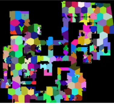
Fig. 1. Region partitioning of an example grid map (73 states, ).
Fig. 2. Region partitioning of an actual game map (9 762 640 states, ).
region construction. The agent then executes the resulting plan in reverse, thereby traveling from the record’s end to the global goal. The cost of this optimization is that it increases the move time, specifically the last moves, as the algorithm may need to perform two hill-climbing checks of up to steps. This would increase the average move time only when used.
On the four-region example, shown in Fig. 1, the two opti-mizations work as follows. For thefirst optimization, consider state before it is added to region . Sup-pose that at this point, all states in the region within three or fewer steps from the representative (2, 4) have been added to the region. Without the optimization, we would hill climb from (2, 8) to (2, 4) andvice versato determine whether we can add (2, 8) to region 1. With thefirst optimization, hill climbing is terminated as soon as state (2, 7) is reached. State (2, 8) is then added to the region since we reached (2, 7) in one step and it is three steps away from the representative. The sum
is less than the cutoff . The second optimization avoids the hill-climbing check from (2, 4) to (2, 8) entirely. Then, on-line, the agent is guaranteed to be able to travel from (2, 4) to (2, 8) by planning a hill-climbing path from (2, 8) to (2, 4) and then executing it in reverse. An example of the regions built for an actual map is in Fig. 2.
2) Abstraction Indexing: The mapping of base states to ab-stract regions must be stored to identify which region each base
state is in. In the worst case, this can occupy the same amount of space as the search space. In practice, performance can be im-proved by compressing the mapping using run-length encoding (RLE) into an array sorted by a state identifier (a unique scalar). On a grid map, a cell is assigned its identifier (id) as
( is the map width).
For the map in Fig. 1 the representatives are , (2, 9), (7, 2), (7, 7), which, with , translate to ids: 26, 31, 79, and 84, respectively. The RLE compression works by scanning the map in row order and detecting changes in abstract region indices. Thefirst record added to the table is (12, 1) since , and the state is assigned to region 1: . Thefirst change of region index happens at state (1, 7), which belongs to region 2. As , record (18, 2) is added to the table. The next region change is detected at (2, 1), adding (23, 1) to the table. Once the compressed records are produced, the original abstraction mapping is discarded.
The RLE table contains at least records where is the number of abstract regions. As it is sorted by state id, the worst case time to map a state to its region is . Ob-serve that may increase with the total number of states (which happens, for instance, in video-game pathfinding if isfixed). To get amortized constant time independent of (as necessary for real-time performance of HCDPS2), we use a hash index on the RLE table. The index maps every th state id to its corresponding record in the RLE table. To look up re-gion assignment for state , wefirst compute the hash table index as . We then run linear search in the RLE table starting with record number until wefind a record with state id exceeding (or equal to) . If
, then . Otherwise , the
region is indicated in the immediately preceding RLE record. The query time is , where is independent of .
3) Computing Paths Between Seeds With Dynamic Pro-gramming: At this point, we have partitioned all states into abstract regions and recorded the region representatives as hill climbing reachable from all states in their regions. We will now generate paths between any two distinct region representatives. First, we compute optimal paths between representatives of neighboring regions, up to regions away. This is done by running A in the search space. The costs of such base paths are used to populate an cost matrix for paths between all region representatives. We then run the Floyd–Warshall algorithm [16], [17] on the matrix. The algorithm has a time complexity of and computes all weights in the matrix. Note that due to the abstraction this problem does not exhibit optimal substructure. Specifically, an optimal path between a representative for the region and a representative for the region may be shorter than the sum of the optimal paths between and and between and , even if the path passes through the region . Thus, the computed paths are approximations to optimal paths.
Once dynamic programming is complete for each region, we will know the next region to visit to get to any other region.
2The standard practice in real-time heuristic search is to accept amortized
This is similar to a network routing table which stores the next hop to get to any network address. With this table, it is possible to build a path between any pair of region representatives by starting at one region representative and continually going to the specified next neighbor. Since as an initial step we generated optimal paths between neighboring regions, we can assemble these into approximately optimal paths between more distant regions.
From an implementation perspective, there are several key issues. First, by increasing , we can get more optimal solu-tions by directly computing more base paths. Two regions and are immediate neighbors if there exists an
edge with and . By scanning the
search space, an abstraction space can be produced with nodes being each region and edges connecting neighboring regions. Then, the neighbors away from a given region are all the nodes reachable from the given region’s node by traversing up to edges. At the limit, , in which case dynamic pro-gramming is not used at all, and we have exact paths between all region representatives. Clearly, the time increases with . A second issue is that if the number of regions is large, the actual implementation structure would be an adjacency list rather than a 2-D array as the matrix is sparse. This saves space and allows the algorithm to be useful for search spaces with larger numbers of regions. Third, it is possible to have variations of the algo-rithm which either materialize all paths or produce them only on demand. It is also possible to have a non-real-time version of the algorithm that only computes the base paths and saves the dynamic programming step for the online stage. We discuss such variants in Section VI.
To illustrate, using the example in Fig. 1 with , we
first compute optimal paths between immediately neighboring regions (i.e., 1 2, 2 4, 3 4). The costs of the resulting
paths are put in an matrix
(1)
Costs of longer paths (e.g., between regions 1 and 3) are then computed with the Floyd–Warshall algorithm. The resulting cost matrix for all region pairs is
(2)
4) Database Record Generation: Once we have approxi-mate optimal paths between all pairs of regions, we compress them into subgoal records. This is done to reduce the space complexity of the database. Specifically, given an actual path , we initialize a compressed path by storing the beginning state of in it. We then use binary search tofind the state such that is not hill climbing reachable from the end state of but the immediately preceding state
is. We then add to and repeat the process until we reach the end state of which we then add to as well. Each com-pressed path becomes a record in our database. Online, each
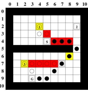
Fig. 3. Start and end optimizations.
element of such a record is used as a subgoal. An example of a compressed path is shown in Fig. 3. In this example, the com-pressed path consists of only the start (S) and goal states (G) and one subgoal at (6, 8).
Note that the subgoals are selected only to guarantee that each subgoal is hill climbing reachable from the previous one in the record. However, such reachability does not guarantee cost opti-mality. Consequently, online, an agent may have a nonzero sub-optimality even if it is solving a problem whose compressed so-lution is already stored in the database.
5) Database Indexing: The offline stage finishes with building an index over the database records to allow record retrieval in constant time. A simple index is an matrix that stores the compressed paths between pairs of regions: entry stores the database record from the region representative to the region representative .
B. Online Stage
Given a problem , HCDPS first seeks the re-gions in which its start and goal states are located. Suppose is located in a region with representative and is located in a region with representative . By re-gion construction, the agent can hill climb from to and travel from to without state revisitation. Furthermore, the agent’s database contains a record with subgoals connecting and . Thus, the agent hill climbs from to , then be-tween the subgoals all the way to , and then, to . Thus, the maximum move time is equal to the time to look up the record to use during thefirst move. After that point, the move time is the time for performing greedy hill climbing to the next state.
There are several enhancements to this basic process, de-signed to improve solution optimality at the cost of increasing planning time per move. None of these optimizations affect the hard cap for move time as the agent always plans itsfirst step to the next subgoal from the database record before attempting the optimizations. This is used if the time runs out before any of the optimizations complete.
Fig. 4. Generalized optimizations.
runs out of the move quota before reaching , then we go to thefirst subgoal in the database record as usual.
Second, when we do use a record, we check if itsfirst subgoal (i.e., the state following in the record) is hill climbing reach-able from . If so, then we direct the agent to go to thefirst subgoal instead of the record’s start. The same move-capped hy-pothetical hill-climbing test is used here. Likewise, when the agent reaches the subgoal before the end of the record , it checks if it can hill climb directly to .
A generalization of these start and end hill-climbing checks is as follows. Consider a case where it is not possible to hill climb from to thefirst subgoal , in the database record with start . We know from construction that it is possible to hill climb from to . Suboptimality can be improved if we canfind the farthest state on the path from to , where we can hill climb from to and from to . The state can be found byfirst reconstructing the path from to (using hill climbing) and then considering the states on this path from toward . For each such state , we try to plan a hill-climbing sequence from to . If we succeed in under moves, then we set to and terminate the search. Once is computed, the agent hill climbs from to . A similar optimization is applied at the end of the record, except the objective is tofind the closest state to the second-last state of the record from which the agent can hill climb to .
The optimizations are illustrated in Figs. 3 and 4. The agent starts out in state with the goal of arriving at . The empty circles are states visited by an HCDPS agent without the online optimizations, and thefilled circles are states visited with the optimization. Light/yellow shaded cells are subgoals from the database record the agent is using. Dark/red shaded cells are reconstructed by hill climbing. For this example, assume that the database was computed with , but the value of does not affect the example as a record is computed between all regions either directly or using dynamic programming.
In Fig. 3, the problem is to navigate from the start
to the goal (6, 4). The start is in region 2 and the goal is in region 3, so the database contains a record between the region representatives (2, 9) and (7, 2). The record contains three states: (2, 9), (6, 8), (7, 2). The online algorithm without optimizations navigates from (2, 7) to the start of the record (2, 9). The next subgoal is (6, 8), so the algorithm hill
climbs from (2, 9) to (6, 8) and then onto the end of the record (7, 2). Finally, it hill climbs to the goal (6, 4).
The start optimization will try to hill climb from the problem start (2, 7) directly to the second state in the record (6, 8), which is successful. The end optimization will try to hill climb from the second-last state in the record [also (6, 8)] to the goal (6,4), which is also successful. These two optimizations reduce sub-optimality from 57% to 0%. In Fig. 4, an HCDPS agent is navi-gating from the start (4, 5) to the goal (9, 3). The start is in region 1 with the representative (2, 4). The goal is in region 3 with (7, 2). The agent locates a database record [(2, 4), (6, 8), (7, 2)].
The start optimization attempts to hill climb from the start state (4, 5) to the second state in the record (6, 8), but fails as hill climbing terminates at (4, 8) due to reaching a local minimum. The generalized version of the start optimization is then tried where the algorithm tries to determine the state farthest along the reconstructed path from the record start (2, 4) to (6, 8) that is hill climbing reachable from the start (4, 5). The searchfinds the state (5, 9), to which the agent then hill climbs from its start state. Once at (5, 9), it continues with the record, hill climbing to (6, 8).
The end optimization check from (6, 8) to the goal (9, 4) ter-minates as the goal isfive states away and the cutoff is . Thus, the generalized version of the end optimization is per-formed to locate the closest state to (6, 8) from which the agent can hill climb to its global goal of (9, 3). The agentfirst recon-structs (via hill climbing) a path from (6, 8) to the end of the record (7, 2). It then tries states on the path and locates (7, 7), from which it can hill climb to (9, 3). As a result of these two optimizations, path suboptimality is reduced from 74% to 0%.
VI. ALGORITHMVARIATIONS
Some of the steps performed offline can be moved online or avoided completely to save offline computation time. We present four variations of HCDPS that make such tradeoffs.
A. HCDPS: Basic Version
The basic version of HCDPS described in Section IV per-forms the abstraction, dynamic programming, and complete database path generation during the offline phase. There are a few issues with the basic version. The abstraction may produce a large number of regions . This reduces performance in two ways. First, during dynamic programming, the time complexity is , and a 2-D matrix implementation has the space complexity of . Even more costly, all paths are enumerated and stored in the database, which is expensive in time and space. In practice, once becomes greater than several thousand, it is not possible to construct and store the entire database in memory.
B. dHCDPS: Dynamic HCDPS
with A for neighboring regions. dHCDPS forgoes this path as-sembly step offline and, instead, stores only the distance table and the optimal paths between the neighboring regions. Since paths between distant regions are not computed offline, there is no need to compress them. Only the paths between neighboring regions are compressed. Then, online, dHCDPS uses the dis-tance table tofind the next region to travel to and follows the correct optimal path to it. This is slightly more expensive com-pared to HCDPS, as the database lookups are more frequent, but the offline phase is accelerated.
C. nrtHCDPS: Non-Real-Time HCDPS
nrtHCDPS is a non-real-time version that performs the dy-namic programming step online on demand. This is done by computing the optimal neighbor paths and storing their costs, as done in the other versions. Dynamic programming is not per-formed at all in the offline phase. Rather, the database consists of only the optimal paths between neighbors and their costs. On-line, if the path required is not a neighbor path, it is constructed by running Dijkstra’s algorithm over the abstract space. Specifi -cally, the database contains a representation of the abstract space where each vertex is an abstract region and each edge is a com-puted cost between neighbors’ representatives. Dijkstra’s algo-rithm is run on this graph to compute the optimal path between a particular start and goal vertex (abstract regions). Given this solution path, the path in the base space is produced by taking each edge in the abstract solution (which maps to a compressed base path) and combining them. Our implementation uses Dijk-stra’s algorithm to search the abstract space, but A and other algorithms are also possible.
Since the dynamic programming time, even when solving a single problem rather than computing the whole table, depends on (and hence indirectly on ), the real-time constraint is violated. The advantage is that the costly dynamic programming step is avoided offline and is performed only when necessary online. We compare nrtHCDPS to other non-real-time search algorithms in the empirical evaluation.
D. A DPS
Instead of using hill climbing as the base algorithm, this ver-sion uses A with ana prioriset limit on the number of states ex-panded per move [denoted by capped A (cA )]. In other words, both offline and online, we run A which expands up to a certain number of states from the current state and then travels toward the most promising state on the open list.
This is different from TBA in two ways. First, A DPS does not retain its open and closed lists between the moves, which makes it incomplete with respect to the global goal. Complete-ness is restored by using subgoals. The subgoals are selected such that each is reachable by cA from the previous subgoal. Likewise, the regions are built using cA -reachability checks, and, hence, each state in a region is cA -reachable to/from the representative.
The rest of the HCDPS implementation and all of its opti-mizations stand with one exception. Specifically, recall that the regular version of HCDPS can terminate its hill-climbing check from a candidate state to a region representative as soon as a state already in the region is reached. A DPS cannot do so
be-cause reaching a state when building its open list does not mean that the state will be the one to which cA will move when it reaches its state expansion limit.
The advantage of A DPS is that the regions can be larger since cA is more robust with respect to heuristic depressions than hill climbing. cA can produce regions of arbitrary size by controlling the cutoff, whereas hill-climbing abstraction has a fundamental upper bound on region size that depends on the map topology. That is, increasing the cutoff for hill climbing will eventually have no effect as the hill-climbing algorithm will terminate due to hitting plateaus rather than by hitting the cutoff. Larger regions lead to a lower number of them , hence speeding up the offline part as well as reducing the database size. On the down side, running A can be slower than hill climbing per move, which slows down region partitioning. The lack of the aforementioned region-building optimization further com-pounds the problem. The tradeoff is investigated in Section VIII.
VII. THEORETICALANALYSIS
In this section, we theoretically analyze HCDPS’ properties and present the results as a series of theorems. We start with the notation used in this section. is the total number of states in the search space, is the number of regions the abstraction procedure produces using a cutoff on moves. is the depth of the neighborhood used to compute optimal paths between re-gion representatives. Any two rere-gions more than regions apart will have the path between their representatives approximated by dynamic programming. If and are states, then is the cost of an optimal path between them and is the number of edges in such a path. is the maximum branching factor in the search space (i.e., the maximum out-degree of any vertex). is the maximum branching factor in the space of regions (i.e., the maximum number of regions adjacent to any region). is the diameter of the space (i.e., the longest shortest path among any two vertices, measured in the number of edges). is the number of base states represented by one index entry in the RLE array (Section V-A2). All proofs apply to the basic version of HCDPS. Behavior of other versions is discussed in Section VI.
Lemma 1 (Guaranteed Suitable Record): For every pair of states and (such that is reachable from ) there is a record in the HCDPS database that the algorithm can hill climb to and hill climb from.
Proof: All proofs are found in the Appendix.
Lemma 2 (Guaranteed Hill Climbability Within a Record): For each record (i.e., a compressed path), itsfirst subgoal is hill climbing reachable from the path beginning. Each subgoal is hill climbing reachable from the previous one. The end of the path is hill climbing reachable from the last subgoal.
Lemma 3 (Completeness): For any solvable problem (i.e., a start and a goal states that are reachable from each other), HCDPS willfind a path between the start and the goal in afi -nite amount of time without any state revisitation between its subgoals.
Theorem 1 (Offline Space Complexity): The total worst case space complexity of the offline stage is .
Theorem 2 (Offline Time Complexity): The worst case
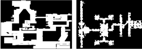
Fig. 5. Two of the 14 maps used in our empirical evaluation.
Theorem 3 (Online Space Complexity): Let be the number of agents searching the same graph that share the database. Then, the worst case online space complexity per agent is
.
Lemma 4 (Real-Timeness): The worst case online amortized time complexity is .
Lemma 5 (Maximum Number of Regions): If the search space is nonempty, then with both bounds tight even
for .
Theorem 4: If the start and goal states fall into abstract re-gions at most regions apart, then the worst suboptimality is upper bounded by a linear function of the product of the region cutoff and the ratio of the smallest and the largest edge
costs: .
Corollary 1: If the conditions of Theorem 4 hold and the goal is at least edges away from the start, then the worst case suboptimality upper bound does not depend on .
VIII. EXPERIMENTALRESULTS
The HCDPS algorithm was compared with D LRTA , kNN LRTA , TBA , weighted A , LSS LRTA , LRTA with sub-goals, BEAM, and the minimal-memory version of PRA [8] for video-game pathfinding. Two sets of maps were used for ex-perimentation (Fig. 5). Thefirst set of game maps are modeled afterCounter-Strike: Source[18], a popularfirst-person shooter. These four maps have between 9 and 13 million states. We used 1000 randomly generated problems across the four maps (i.e., 250 per map). For each problem, we computed an optimal so-lution cost by running A . The optimal cost was in the range of [1004, 3000] with a mean of 1882, a median of 1855, and a stan-dard deviation of 550. We measured the A difficulty, defined as the ratio of the number of states expanded by A to the number of edges in the resulting optimal path. For the 1000 problems, the A difficulty was in the range of [1, 199.8] with a mean of 62.60, a median of 36.47, and a standard deviation of 64.14.
We also tested the algorithms on ten of the largest standard benchmark maps fromDragon Age: Originsavailable at http:// movingai.com. The ten maps selected werehrt000d,orz100d, orz103d,orz300d,orz700d,orz702,orz900d,ost000a,ost000t, andost100d. These maps have an average number of open states of 96 739 and total cells of 574 132. For each map, we selected the 100 longest sample problems from the problem set. The op-timal cost was in [407, 2796] with a mean of 1270, a median of 1039, and a standard deviation of 618.
Algorithms were tested using Java 6 under SUSE Linux 10 on an Intel Xeon E5620 2.4-GHz processor with 24 GB of memory. All timings are for single-threaded computations.
HCDPS was run for neighborhood depth . The base version of HCDPS as well as dHCDPS and nrtHCDPS were tested. We also tested HCDPS and dHCDPS with
, which computes exact paths between all regions rather than using dynamic programming. D LRTA was run with clique abstraction levels of {9, 10, 11, 12} for theCounter-Strikemaps and {6, 7, 8, 9} for theDragon Agemaps. kNN LRTA was run with database sizes of {10 000, 40 000, 60 000, 80 000} records. We used steps for hill climbing and for RLE indexing forCounter-Strike, and and
forDragon Age. kNN LRTA used reachability checks on the ten most similar records. TBA was run with the time slices of {5, 10, 50, 100, 500, 1000, 10 000} states expanded. Its cost ratio of expanding a node to backtracking was set to 10. LSS LRTA was run with the number of states expanded as {10, 100, 1000, 10 000}. LRTA with subgoals had no configuration parameters. Note that we improved the implementation of this algorithm to select its first subgoal as the closest subgoal by heuristic distance that is hill climbing reachable. Without this reachability check, the suboptimality of the algorithm is over 10% higher. The real-time algorithms were also compared with non-real-time algorithms, including weighted A with weights of {2, 5} and BEAM with beam widths of {10, 50, 100}. PRA was run with grid (sector) sizes of 16 16, 32 32, 64 64, and 128 128.
We chose the space of control parameters with three consid-erations. First, we had to cover enough of the space to clearly determine the relationship between control parameters and algorithm performance. Second, we attempted to establish the Pareto-optimal frontier (i.e., determine which algorithms dominate others by simultaneously outperforming them along two performance measures such as time per move and subop-timality). Third, we had to be able to run the algorithms in a practical amount of time.
A. Database Generation
1) Counter-Strike Maps: Two important measures for data-base generation are generation time and datadata-base size. Genera-tion time, although offline, is important in practice, especially when done on the client side for player-made maps. Database generation statistics are given in Fig. 6.
Fig. 6. Generation time versus space forCounter-Strikemaps.
LRTA and kNN LRTA that are small and fast, these databases have too high a suboptimality when used.
Varying the number of neighbor levels for HCDPS increases the database generation time and size. This additional time is solely related to A time in computing optimal paths between region representatives. Abstraction time and dynamic programming times are unchanged. This additional A time computing optimal neighbor paths improves suboptimality, which is discussed in Section VIII-B. For HCDPS, an L2 database is generated in 110 s with size 1.1 MB, compared to a time of 22 s and 13 KB for DHCDPS L2. For HCDPS, an L4 database is generated in 590 s with size 1.1 MB, compared to a time of 342 s and 110 KB for DHCDPS L4.
A DPS abstraction with the same produces more abstract regions, which results in a larger database. This is due to the fact that the cutoff limits the number of states expanded in A DPS as opposed to the number of states traveled in HCDPS. Con-sequently, the regions produced by A DPS tend to be smaller than those produced by HCDPS for the same value of . The A DPS abstraction also consumes significantly more time due to A being a substantially slower algorithm than hill climbing and the early termination optimization (which remembers states in the region when building regions) cannot be used. Interest-ingly, the overall time increases as the region size gets larger. This is due to two factors. First, the abstraction time increases as each reachability check takes longer. This is a major factor in the time for A DPS. Second, the time to produce the base neighbor records grows significantly as these are computed by A , and the paths between regions become longer (more states expanded) as the regions become larger. The results show that using A as a reachability check algorithm is inferior to simple hill climbing.
PRA produces no database of records, so its time only relates to the abstraction time. Abstraction time is very short as the map is divided into sector grids, and regions are built only within sector boundaries.
The two HCDPS offline optimizations improve performance. The one-way optimization that only performs the hill-climb check to the region representative reduces the time by about
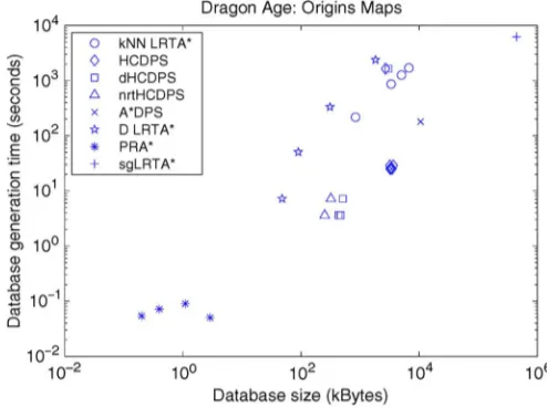
Fig. 7. Generation time versus space forDragon Agemaps.
a factor of 2, and the optimization to remember states in the region to allow early termination when hill climbing to the representative reduces the time by a factor of approximately 20. Not performing the hill-climbing check from the representative to a candidate state has a further advantage of creating larger regions as more states are eligible for inclusion into the region. This reduces the number of overall regions, the generation time, and database size.
2) Dragon Age Maps: The database generation results for Dragon Agemaps are in Fig. 7. These results follow the same trend as the Counter-Strikemaps despite the maps being two orders of magnitude smaller. All versions of HCDPS can build the database in less than 30 s. dHCDPS can produce a database in less than 5 s and uses less than 500 KB. These results are two orders of magnitude smaller than D LRTA and kNN LRTA . HCDPS is three orders of magnitude faster than LRTA with subgoals (sgLRTA ), and its database is 100 times smaller. The reason is that sgLRTA builds a tree record for every open state in the map which requires visiting every state via Dijsktra’s al-gorithm. PRA has a smaller precomputation size as no database records are generated, and it does not store an explicit mapping between abstract and base states.
B. Online Performance
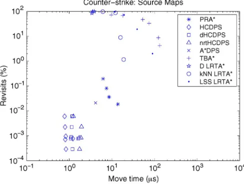
1) Counter-Strike Maps: The online performance is mea-sured with several metrics, including suboptimality versus move time (Fig. 8), number of revisits versus move time (Fig. 9), and suboptimality versus total memory usage (Fig. 10). Total memory usage includes the space for the database and online memory used for one agent pathfinding.
Fig. 8. Suboptimality versus move time forCounter-Strikemaps.
Fig. 9. Revisits versus move time forCounter-Strikemaps.
Fig. 10. Memory versus suboptimality forCounter-Strikemaps.
when allowed to expand more states per time slice. HCDPS and dHCDPS are similar in suboptimality. A DPS with
produces smaller regions than the hill-climbing-based ver-sions and turns in a higher suboptimality and slower times than HCDPS. Although in general smaller regions improve
subopti-TABLE I
EFFECTS OFONLINEOPTIMIZATIONS
mality, cA compressed paths have more subgoals to cover the same distance on the map.
For move time and overall time, HCDPS is superior to all algorithms by a factor of 1.5 to 3. D LRTA move time is low as it only needs to look up the next subgoal in its abstraction table. However, its overall solution time is high as the paths produced are more suboptimal and contain more moves. kNN LRTA ’s move time increases based on database size as it must identify the best record by searching all records. TBA with a small time slice can have low move times at the cost of substantially higher suboptimality. However, its overall planning time is relatively long. The base version of HCDPS has the lowest move time as it simply must follow a completed record. dHCDPS takes slightly longer as it must reconstruct the record from fragments, and nrtHCDPS is slightly longer still as it must compute the shortest path for the problemfirst, and then reconstruct the path from fragments.
We have also experimented with the effect of removing the optimizations that HCDPS applies. The effects of these optimizations on dHCDPS are shown in Table I where we compare no optimizations (“none”), with only the start optimization (“start”), only the end optimization (“end”), both (“start+end”), and start and end together with their generalized versions (“all”).
3) Comparisons to Non-Real-Time Algorithms: In compar-ison to the non-real-time algorithms BEAM, and weighted A , nrtHCDPS has lower suboptimality and a faster overall time by at least ten times. The move time for these algorithms is calcu-lated as the overall time, divided by the length of the path (time per move). However, the response time of these algorithms is approximately the same as their overall time, as a complete path needs to be generated before any move is taken. nrtHCDPS has the best overall planning time, approximately 60 times faster than A , 10 times faster than weighted A (with the weight of 5), and about 20 times faster than BEAM search.
The amount of memory consumed to perform one A search is higher than that used by the database for nrtHCDPS. Further, this memory is needed for each A agent, where the database is shared among multiple agents operating on the same map. Ad-ditionally, the HCDPS database is read-only, which is advanta-geous on certain hardware such asflash memory.
Fig. 11. Suboptimality versus move time forDragon Agemaps.
no database is constructed. With 16 16 tiles, its suboptimality is superior, but running A on the abstract space takes more time and space for thefirst move. There is no overall winner between the two algorithms with each algorithm making different trade-offs and having its own strengths. Note that for HCDPS its on-line memory usage is zero, so any number of agents pathfinding simultaneously consume the same amount of memory as one. HCDPS only uses space for its database. For PRA , the on-line memory usage is between 20 and 400 KB depending on the problem. So, HCDPS will be superior in memory usage when tens of agents are pathfinding simultaneously. For PRA 16 16 compared to nrtHCDPS L3, the cutoff isfive agents where nrtHCDPS would consume less total memory.
C. Dragon Age Maps
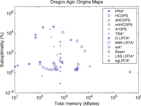
The online performance results for theDragon Agemaps are in Figs. 11–13. These results are similar to the results of the Counter-Strikemaps. By three levels of neighbors, all versions of HCDPS are under 3% suboptimality and, overall, times two orders of magnitude faster than all other real-time algorithms. The poor coverage issues are even more dramatically apparent with D LRTA and kNN LRTA . For D LRTA , less abstraction (levels 6 and 7) actually turn out worse than levels 8 and 9. This variability is due to the complex structure of the abstraction re-gions, which can cause the algorithm to effectively degenerate to LRTA while navigating out of a region with a large heuristic depression. For kNN LRTA , even a large database does not guarantee overall good performance. In spite of its 80 000 record database, it only takes one problem to prevent kNN LRTA from
finding a hill climbing reachable record, and the average sub-optimality increases substantially. HCDPS clearly outperforms all algorithms that perform precomputation of subgoals, except for LRTA with subgoals (extended with a hill-climbing reach-ability check).
Comparing TBA and LSS LRTA shows that TBA dom-inates LSS LRTA in all categories. For the same number of states expanded, TBA has lower suboptimality and a faster time per move. The suboptimality for TBA and LSS LRTA for such a small number of states expanded is substantial.
Fig. 12. Revisits versus move time forDragon Agemaps.
Fig. 13. Total memory versus suboptimality forDragon Agemaps.
sgLRTA has a very low suboptimality (assuming the al-gorithm is modified to set thefirst subgoal to be the closest, hill-climbing reachable subgoal) as it stores a state to exit every heuristic depression. Thus, although the database computation time and size is large, this does pay off online in terms of per-formance. It is slower on average move time as it uses LRTA as a base algorithm, which has higher overhead than simple hill climbing.
Finally, although HCDPS does not completely eliminate re-visits, the percentage is low (less than 0.08% in all cases), which is a significant improvement over previous algorithms.
D. Summary of Results
In the following, we summarize the performance results of the algorithms.
Suboptimality versus move time is dominated by HCDPS for real-time search algorithms. It has lower suboptimality than all other real-time algorithms, except for the modified LRTA with subgoals algorithm, TBA , and LSS LRTA with high cutoff limits. All these algorithms take longer per move. HCDPS is clearly superior to the other subgoaling solutions such as D LRTA and kNN LRTA , which are fragile and can produce very suboptimal solutions. Being robust is important to video-game pathfinding as a single outrageously suboptimal path can break a player’s immersion. The comparison with PRA is mixed. Depending on the maps, PRA may have higher or lower suboptimality but its move times are always longer.
Revisits versus move time is dominated by HCDPS for all real-time algorithms. Its move times are the fastest, and its re-visits are the lowest. A and its variants have no rere-visits but longer move times.
Database generation time and spaceis dominated by PRA as it stores only a small abstraction which takes little time to produce. HCDPS is faster than all other real-time abstraction ap-proaches. Clearly all the nonprecomputation algorithms (TBA , LSS LRTA , A ) dominate this metric as they require no pre-computation at all. Although a kNN LRTA or D LRTA data-base may be smaller than HCDPS, those datadata-bases do not cover the space adequately resulting in unacceptably high subopti-mality. Database size for abstraction techniques like PRA and HCDPS depends on both the map size and its complexity.
Suboptimality versus total memory usageis the fundamental tradeoff with no clear winner. HCDPS dominates previous real-time algorithms as it has a lower suboptimality for memory used. sgLRTA has lower suboptimality than HCDPS as it stores more information in its database. It also allows for guaranteed coverage and low maximum suboptimality. However, its data-base construction time becomes too long (square in number of states) as the map gets larger, and the database size becomes impractical. PRA has a lower memory usage than HCDPS but may or may not be superior for suboptimality depending on the map. Further, as more agents are simultaneously pathfinding, HCDPS will use less total memory as its per-agent memory usage is zero.
IX. CURRENTSHORTCOMINGS ANDFUTUREWORK
HCDPS is an efficient algorithm for grid pathfinding on video-game maps, but there are several limitations to its gen-eral application to other search problems. First, the algorithm must be able to efficiently enumerate all states in the search space to perform the abstraction. Consequently large implicitly specified search spaces (e.g., the 24-tile sliding tile puzzle) are out of reach for HCDPS. Second, even if HCDPS is able to enu-merate all states, the resulting number of regions has to be small as the computational complexity is at least cubic in the number of regions. For instance, the maps used in our experiments had millions of states, which resulted in a few hundred abstract regions. This is because the region representatives were hill climbing reachable from a large number of states. Should the
topology be more complex relative to the heuristic function, the hill climbing will fail more often, reducing the region size and thus increasing the number of regions. dHCDPS and nrtHCDPS reduce precomputation and thus push the boundary further but will eventually become intractable. We have conducted some initial experiments in other domains including mazes. The major challenge with mazes is that the abstract regions are quite small, which results in a larger database size.
The other limitation common to all precomputation ap-proaches is the static search space assumption. Changes to the search space (e.g., a bridge is built on a video-game map) re-quire changes to the database. Recomputing the entire database online for each change may be too slow.
Future work will tackle these limitations. Partial partitioning may be used for spaces which are too large to partition fully. A hybrid of kNN LRTA ’s random database and HCDPS sys-tematic database may be fruitful as well. Future work will com-pare the uniform placement of region representatives with using Voronoi diagram regions. It is also possible to investigate the approach in comparison to other game navigation approaches, such as potentialfield-based navigation and using HCDPS with navigation meshes.
X. CONCLUSION
In this paper, we have presented HCDPS, thefirst real-time heuristic search algorithm with neither heuristic learning nor maintenance of open and closed lists. Online, HCDPS is simple to implement and dominates the current state-of-the-art algorithms by being simultaneously faster and better in solu-tion quality. It is free of both learning and the resulting state revisitation which prevents all previously published real-time search algorithms from being used in games. This performance is achieved by computing a specially designed database of subgoals. Database precomputation with HCDPS is two orders of magnitude faster than kNN LRTA and D LRTA . Finally, its read-only database gives it a smaller per-agent memory footprint than A or TBA with two or more agents. Overall, we feel HCDPS is presently the best real-time search algorithm for video-game pathfinding on static maps.
APPENDIX
Proof of Lemma 1:For , there is a representative state reachable from via hill climbing. Likewise, for state , there is a representative state such that can be hill climbed to from . This follows from the way the state space is partitioned and the way the region representatives are identified during the database construction.
Proof of Lemma 2: This is guaranteed by record construc-tion.
a state visited on the climb from to can be revisited on the climb from to .
Proof of Theorem 1: The number of compressed paths in the database is . Each path is at most states, where is the diameter of the space and hence the worst case data-base size is . Mapping between all states and their regions adds space where is the number of states. Thus, the total worst case space complexity is .
Proof of Theorem 2: While forming a region with a cutoff , each candidate state is required to be fewer than hill-climbing steps away from the representative state. Hence, the maximum number of candidate states in a region with a cutoff of and the maximum branching factor of is . Each candidate state takes no more than hill-climbing steps to check if it is bidirectionally hill climbing reachable with the representative state. Hence, the total number of hill-climbing steps needed to form a region is . No state can be assigned to more than regions. Hence, the worst amount of work per all states in the largest region is hill-climbing steps. Since there are regions, the total number of hill-climbing steps to partition all states is .
A is run for no more than problems. Thus, the total run time is in the worst case. Running dynamic programming takes . Each of the resulting paths requires no more than to compress, as there are no more than subgoals in each path and each subgoal takes at most hill-climbing checks of no more than steps each. Building the compressed mapping table requires a scan of the map and is . Hence, the overall worst case offline complexity is
.
Proof of Theorem 3: HCDPS takes space per state per agent for hill climbing. However, it needs to load the data-base and the index resulting from the total space complexity of . Note that the database is shared among of simultaneously pathfinding agents. Thus, per agent, worst case space complexity is
.
Proof of Lemma 4: On each move the agent expands its current state, incurring the time expense of . Tofind a database record for thefirst move, it uses a hash table. Thus, the database query time is .
Proof of Lemma 5: Since the abstract regions partition the space of states, trivially holds. Clearly,
when , which makes both the upper and lower bounds tight. We will now show that it is also possible that or even if . The case of , , is easily achieved when, for instance, the set of states is , and are mutually hill climbable, and the hill-climbing cutoff is above 1. Then, both states will be included in a single region,
making .
Making is possible for an arbitrarily large if the heuristic is 0 everywhere. Then, no state is hill climbing reachable from any other state. Consequently, every single state becomes its own region, resulting in .
Fig. 14. To the proof of Theorem 4.
Proof of Theorem 4: Consider the graph in Fig. 14. The start state is , and the goal state is . falls into an abstract region with the representative state . falls into an abstract region with the representative state . We willfirst consider the case when the two abstract regions are different.
The region construction cutoff is edges, which also serves as the cutoff on the number of edges hill climbed in online checks. From this, we derive:
. Because any edge has the cost of at most , we have: . Since has at least one
edge, .
Since the two abstract regions are within regions apart, the path between and is optimal. Therefore,
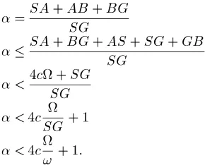
. In order for HCDPS to prefer path to path , the online hill-climbing check from to must fail. This can happen if, for instance, is in a local heuristic depression or on a heuristic plateau. Then, the suboptimality of going through the states and is defined as
We now consider the case when and fall into the same abstract region. As every region has a single representative state,
. Then, the suboptimality of traveling from to to is at worst
In either case, the worst suboptimality is upper bounded by a linear function of the product of and the cost ratio .