INDUNIL DE SILVA AND SUDARNO SUMARTO
TNP2K WORKING PAPER 04 – 2013 December 2013
POVERTY-‐GROWTH-‐INEQUALITY
TRIANGLE:
TNP2K Working Papers Series disseminates the findings of work in progress to encourage discussion and exchange of ideas on poverty, social protection and development issues. Support for this publication has been provided by the Australian Government through the Poverty Reduction Support Facility (PRSF).
The findings, interpretations and conclusions herein are those of the author(s) and do not necessarily reflect the views of the Government of Australia or the Government of Indonesia.
The text and data in this publication may be reproduced as long as the source is cited. Reproductions for commercial purposes are forbidden.
Suggestion to cite: De Silva, Indunil, and Sudarno Sumarto. 2013. “Poverty-Growth-Inequality Triangle: The Case of Indonesia.” TNP2K Working Paper 04 -2013. Tim Nasional Percepatan Penanggulangan
Kemiskinan (TNP2K), Jakarta, Indonesia.
To request copies of the paper or for more information on the series; please contact the TNP2K - Knowledge Management Unit ([email protected]).
Papers are also available on the TNP2K’s website (www.tnp2k.go.id).
TNP2K
Email: [email protected] Tel: 62 (0) 21 391 2812
INDUNIL DE SILVA AND SUDARNO SUMARTO
TNP2K WORKING PAPER 04 – 2013 December 2013
POVERTY-‐GROWTH-‐INEQUALITY
TRIANGLE:
Poverty-Growth-Inequality Triangle:
The Case of Indonesia
Indunil De Silva and Sudarno Sumarto
1December 2013
Abstract
This paper decomposes changes in poverty into growth and redistribution components, and employs several pro-poor growth concepts and indices to explore the growth, poverty and inequality nexus in Indonesia over the period 2002-2012. We find a ‘trickle-down’ situation, which the poor have received proportionately less benefits from growth than the non-poor. All pro-poor measures suggest that economic growth in Indonesia was particularly beneficial for those located at the top of the distribution. Regression-based decompositions suggest that variation in expenditure by education characteristics that persist after controlling for other factors to account for around two-fifths of total household expenditure inequality in Indonesia. If poverty reduction is one of the principal objectives of the Indonesian government, it is essential that policies designed to spur growth also take into account the possible impact of growth on inequality. These findings indicate the importance of a set of super pro-poor policies. Namely, policies that increase school enrolment and achievement, effective family planning programmes to reduce the birth rate and dependency load within poor households, facilitating urban-rural migration and labour mobility, connect leading and lagging regions and granting priorities for specific cohorts (such as children, elderly, illiterate, informal workers and agricultural households) in targeted interventions will serve to simultaneously stem rising inequality and accelerate the pace of economic growth and poverty reduction.
Key Words: Growth, poverty, inequality, pro-poor, decomposition
JEL Classification: D31, D63, I32
1
Senior Economist & Policy Adviser, respectively at The National Team for the Acceleration of Poverty Reduction (TNP2K), Indonesia, Vice-President Office.
1. Introduction
Indonesia, the largest country in Southeast Asia with the world's fourth largest population, is at present using its strong economic growth to accelerate the rate of poverty reduction. Lately, however, in spite of the sustained economic growth, the rate of poverty reduction has begun to slow down, with inequality continuing to rise. Just over the past ten years, as poverty in Indonesia fell by 34 percent, the country’s Gini coefficient rose by around 30 percent. The rising inequalities, attributed to changes in demographics, increased educational attainment and the transformation in the sectoral composition of growth away from agriculture and toward industry and services, are suspected to have dampened most of the poverty-reducing effects of growth. If unattended to, they can further result in forms of collective behaviour that impede economic growth, such as upsurges of social protests seen lately in Indonesia. Even if they do not result in violence, perceptions arising out of inequitable effects of policy reform can increase resistance and undermine the government’s ability to introduce the very important reforms needed for economic growth (Coudouel, Dani and Paternostro 2006).
Indonesia is now facing the twin challenge of accelerating the rate of poverty reduction and at the same time adopting a pro-poor growth framework that allows the poor to benefit more from economic growth, and thereby curb rising inequalities. Policy planners in Indonesia now need to pay special attention to the large and growing inequality, since any attempt to discount the matter will polarise the society, lead to social tensions, and eventually, undermine the growth process itself. Setting targets for greater equity is, however, intricate and not straightforward; complexity should nonetheless not become a pretext for inertia in the face of one of the key development priorities for Indonesia. Thus in this context, it is particularly important to examine the nexus between growth, inequality and poverty in Indonesia from a dynamic perspective.
growth will therefore be larger for higher rates of distribution-corrected growth. More recent studies (Ferreira et al. 2009; Fosu, 2009; Banerjee et al. 2005; World Bank, 2005:2008) have also shown that growing inequality reduces the growth elasticity of poverty reduction, and gives rise to poverty and inequality “traps” that have a detrimental influence on the growth prospects of an economy.
Timmer (2004) investigated the growth process in Indonesia over the 1960-1990 period. His study found that during those three decades, the growth was instrumental in reducing poverty in Indonesia. It further showed how Indonesia has experienced both “relative” and “absolute” pro-poor growth, and concludes that throughout the study period, there have been no episodes in which the poor were absolutely worse off during sustained periods of economic growth. Further, Suryadarma, Suryahadi and Sumarto (2005) showed that high inequality reduced growth elasticity of poverty in Indonesia over the 1999-2002 time period. They found that poverty reduction between 1999 and 2002 was very successful due to inequality in 1999 being at its lowest level in 15 years, thus leading to an increased impact of growth on poverty reduction. In another study, Suryahadi, Suryadarma and Sumarto (2009) further examined the relationship between economic growth and poverty reduction by breaking down growth and poverty into their sectoral compositions and geographical locations. They find that the most effective way to accelerate poverty reduction is by focusing on rural agriculture and urban services growth. Subsequently, Sumarto and Bazzi (2011) found inequality in Indonesia to be historically low relative to other developing countries in Asia and Latin America with large targeted social programmes. They argue that targeting the poor and near-poor is difficult in countries with relatively lower inequality, since the distinctions between poor and non-poor tend to be less sharp, particularly given the clustering of households around the poverty line. Finally, Suryahadi, Hadiwidjaja and Sumarto (2012) assess the relationship between economic growth and poverty reduction before and after the financial crisis in Indonesia. They find that growth in the service sector is the largest contributor to poverty reduction, and that the importance of agriculture sector growth for poverty reduction is confined only to the rural sector.
2. Poverty and Inequality in Indonesia: Initial Conditions
Poverty and Inequality in Indonesia in the regional context
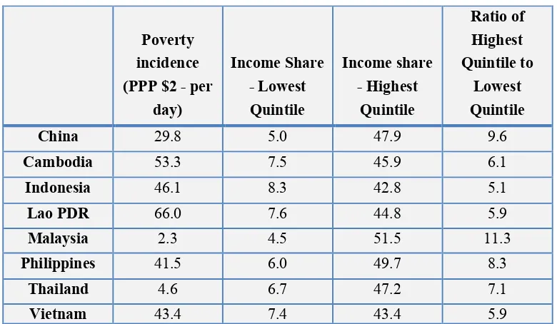
The remarkable success in tackling poverty in East Asia and the Pacific during the past three decades has been associated with an increase in income inequality in several countries in this region. Table 1. Regional Poverty and Inequality gives the regional poverty and inequality profile. According to ADB (2012), several countries in the Asia and Pacific region (such as the People’s Republic of China (PRC), Indonesia, Nepal, Tajikistan, Thailand, Turkmenistan, and Viet Nam) were able to achieve a reduction in poverty incidence of more than 30 percentage points within the last three decades. At the same time, inequality has increased most dramatically in China but has also risen in several other countries such as Indonesia, Mongolia, Vietnam, and Cambodia, at a time when it had been trending downward in many Latin American countries (Figure 1. Change in Inequality, Regional Profile). The Gini coefficient, which measures inequality, recorded new highs of 48.2 percent in China, 45 percent in the Philippines and 40 percent in Thailand, all of which are higher rates than those that prevail in most countries in Eastern Europe and South Asia. Considering the Asia Pacific region as a whole, the Gini coefficient has leapt from 39 to 46 in the last two decades (ADB 2012). Income inequality, as measured by the ratio of income or consumption of the highest quintiles to the lowest ones, also deteriorated in almost half of 30 developing Asian economies, worsening for four of the five most populous countries in the region — Bangladesh, the People’s Republic of China (PRC), India, and Indonesia during the last three decades (ADB 2012).
Poverty and Inequality in Indonesia
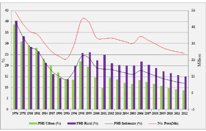
can be deemed as one of the most successful episodes in terms of eradicating poverty, with its incidence declining by three-fold; between 1976 and 1993, poverty declined from 44 percent to 13 percent. Since 1999, poverty headcount index, as measured by the national poverty line, has fallen further in Indonesia.
The period of steady poverty reduction was disrupted by the East Asian crisis, which began July 1997 with the devaluation of the Thai Baht. It was transmitted rapidly to Indonesia with a speculative currency attack on the Indonesian Rupiah. Immediately in August 2007, the Rupiah collapsed and inflation soared, with food prices outpacing general headline prices. A social and economic crisis exploded then into a political one, with the then President Suharto eventually being thrown out of power by mid-1998. By 1998, Indonesia had suffered a multi-dimensional economic and political crisis, triggering the poverty rate to increase from 17 percent in 1996 to 24 percent in 1999. During this period, other socio-economic indicators, such as schooling dropout rate, were also suspected to have increased. However, by 2004 the poverty incidence has been able bounce back again to below pre-crisis levels, at less than 17 percent of the population (Figure 2. Number and Percentage of Poor People in Indonesia).
Later, in 2006, poverty increased again, with the headcount index rising to 17.75 percent from 15.97 percent in the previous year. This time it was primarily due to the government’s policy decision to increase the domestic price of fuel by an average of around 120 percent, and to a sharp increase in the price of rice between February 2005 and March 2006. More recently, in spite of the sustained economic growth, the rate of poverty reduction has begun to slow down. The main reason for this is thought to be the changing nature of poverty. As the poverty incidence approaches a single digit figure and is around ten percent, further reductions in poverty become increasingly more difficult. When the poverty incidence was in mid-twenties, a large number of households used to live just below the poverty line and hence only a slight increase in income was needed to push those households out of poverty. But now the nature of poverty has changed: many households live far below the poverty line and others are clustered just above it, with the risk of falling back to poverty (Suryahadi et al., 2011).
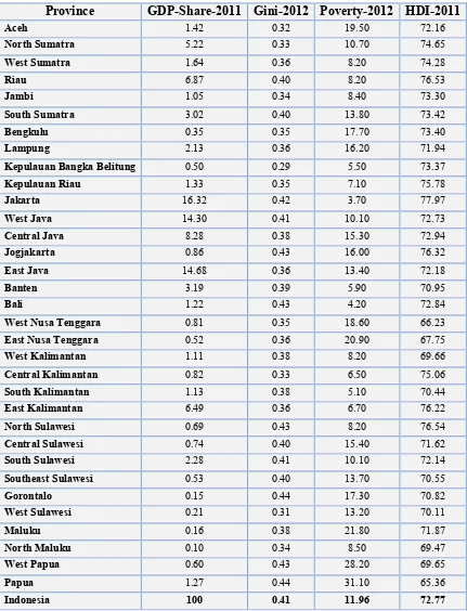
poverty in case of small shocks. Households churning in and out of poverty are thus a very common phenomenon in Indonesia; evidence from panel data suggests that during 2007-2009, more than half of poor in a given year were not poor the previous year. Secondly, the income and monetary poverty measures do not always capture the true picture of poverty in Indonesia; many households who may not be “income poor” could be categorised as multidimensional poor due to lack of access to basic services, employment, education and poor development outcomes. Thirdly, given the vast size of and heterogeneous nature of Indonesian geography, regional disparities are also an entrenched feature of poverty in the country. Indonesia now has 34 provinces, eight of which have been created since 1999. Welfare disparities are significant across these 34 provinces in Indonesia, and national averages mask stark differences. For example, the poverty incidence in some of the outlying provinces such as Papua was as high as 31 percent of the population, as compared to 3.7 in Jakarta in 2012.
Table 2. Regional Socio-Economic Indicators shows the regional output shares in Indonesia together with poverty, inequality and human development indices. Vast disparities that exist between provinces become evident, with provincial income shares varying from 0.1 percent to 16 percent. The Capital of Indonesia, Jakarta, and other resource abundant provinces, such as Riau and East Kalimantan, have remarkably high income shares. It can be also seen that although rates of poverty vary across and within all regions, provinces with low-income shares are mostly in the eastern part of the country. A worrisome feature to note from Table 2. Regional Socio-Economic Indicators is that some western provinces simultaneously exhibit large income shares and high poverty rates.
A widely accepted explanation for the regional output differences is the availability of natural resource prohibitive traffic and high cost of trade among provinces. A more conceivable factor, which is getting broad attention lately, is the structural change that Indonesia has experienced in the past two decades. While the GDP share of agriculture was more than 20 percent in the 1980s, it declined to 15 percent in mid-2000. Meanwhile, the GDP share of the manufacturing sector rose from 16 percent to 26 percent. The trade structure went through an even more radical change as the mining industry lost its dominance of exports. By 2005, the GDP share of non-mining exports amounted to almost 70 percent of total exports. Industrialisation is heavily concentrated, however, in the Greater Jakarta area and export processing zones of Riau Islands. The rising contribution of manufactured goods to the export mix, as opposed to export of such lower-value-added materials as raw lumber and mining ore, thus led to a rapid increase in the GDP per capita in the regions where major investment has been made in manufacturing, leaving other regions lagging behind.
3. Analytical Framework and Methodology
Growth-redistribution decompositions and indices of pro-poorness based on the methodologies of Datt and Ravallion (1992), Ravallion and Chen (2003), Kakwani and Pernia (2000), Kakwani, Khandker and Son (2003) will be primarily be used to examine the dynamics of pro-poor growth in this study. Two different poverty measures that make up the Foster-Greer-Thorbecke (FGT) class were utilised to capture the different dimensions of poverty. The FGT indices combine expenditure and the poverty line in to poverty gaps (PG), and aggregate these gaps to evaluate the extent of poverty. The FGT poverty index can be is the average extra consumption that would be required to bring each poor household up to the poverty line.
The FGT index will be used in this study for both the sectoral and source/component decomposition of poverty. Variables X and Y will be used interchangeably to denote real per capita expenditure that captures the living standard, while Q(p) will be the living standard level below which we find a proportion of p of the population. The sectoral decomposition of poverty by population subgroups/sectors is done by dividing the population in to K mutually exclusive population subgroups and expressing the FGT index as following:
𝑝 𝑧:𝛼 = 𝜙 𝑘 𝑃 𝑘:𝑧:𝛼
the estimated relative contribution of subgroup. Decomposing poverty by subgroups/sectors means that an improvement in one of the subgroups while holding the incomes of the other groups will always improve aggregate poverty. In other words, an independent assessment can be done in the optimal design of social safety nets and benefit targeting within any given subgroup/sector regardless of any other income distributions in other groups. Thus any successful targeting that reduces poverty at the local level implies that poverty at the aggregate level should have also decreased.
The scientific and policy community often tends to define growth pro-poorness based on both absolute and relative approaches. In the absolute approach, growth is defined as pro-poor if there is a reduction in absolute poverty with incomes of the poor rising fast enough to reduce the number of people living below a reference poverty line. The relative approach is based on the notion of whether the incomes of the poor are rising relative to the incomes of the non-poor and hence a decline in inequality. Thus this approach focuses attention on whether the poor are benefiting more or less proportionately from growth and whether inequality, a key determinant of the extent to which growth reduces poverty, is rising or falling over time. Both the relative and absolute concepts of pro-poor growth are equally important, and complement each other in the analysis of growth processes from a pro-poor standpoint. Therefore it is vital that policy planners distinguish between growth that changes the incomes of the poor either by a positive absolute amount (for absolute poverty) and growth that changes the incomes of the poor by the same proportional amount as in the rest of the population (for relative poverty and/or relative inequality).
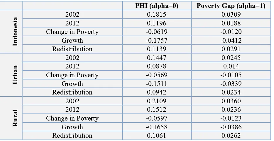
Decomposition of observed changes in poverty between 2002 and 2012 into growth and redistributive components will be based on the methodology of Datt and Ravallion (1992). The change in poverty between 2002 (t-1) and 2012 (t) can be expressed as:
𝑃! 𝑧;𝛼 −𝑃!!! 𝑧;𝛼 = 𝑃!!!
being equal over the period of analysis. The growth term is negative when µμ!>µμ! !!,,
suggesting that growth reduces poverty. Similarly, P! !!!
!!!!;α is the level of poverty in 2012
after its expenditures have been scaled by µμ!!!
µμ! to yield a distribution with mean µμ!!!. The
redistribution effect term is the difference between the two distributions with equal mean expenditures, but different relative expenditure shares. The error term is given by:
𝑃! 𝑧;𝛼 +𝑃!!! 𝑧;𝛼 −𝑃! 𝑧𝜇!
𝜇!!!;𝛼 −𝑃!!! 𝑧𝜇!!!
𝜇! ;𝛼
The error term yields either the difference between the growth effect when using 2012 (t) and 2002 (t-1) interchangeably as reference distributions. Therefore given the path dependence, the error term can be made to disappear by averaging the components (i.e. Shapley
The first pro-poorness measure is the ‘poverty equivalent growth rate’ proposed by Kakwani and Pernia (2000); Kakwani, Khandker, and Son (2003); Kakwani, and Son (2008), which identifies positive growth as pro-poor if the poor benefits proportionately more than the non-poor. The measure is derived from a general class of additively decomposable income-poverty measures which, for a given income-poverty line, z, can be expressed as:
𝜃= 𝑃 𝑧,𝑦 𝑓 𝑦 𝑑𝑦
!
!
where γ=dln(µμ) is the growth rate of mean income and g p =dln(x p ) is the growth rate
of the consumption of people at p-th percentile. Thus δ is the percentage change in poverty headcount resulting from a growth rate of one percent in the mean consumption and is always negative. Next, the growth elasticity of poverty is decomposed in to two components as:
𝛿=𝜂+𝜁
where η=!! !!!"!"y p dp is distribution neutral relative growth elasticity of poverty derived
by Kakwani (1993), and ζ=!"! !!!!!!x p dln L
! p dp is the first derivative of the Lorenz
function L(p) which measures the effect of inequality on poverty reduction. Kakwani et al. (2004; 2008) defines the poverty equivalent growth rate (PEGR)- γ∗, as the growth rate that will yield the same decrease in the poverty headcount as the actual present growth rate γ if the growth process had a zero change in inequality (when everyone in the society had received the same proportional benefits of growth). The actual proportional rate of poverty reduction is equal to δγ, with 𝛿 being the total poverty elasticity. If the growth were
distribution neutral (when inequality had not changed), then the growth rateγ∗ would result in a proportional reduction in poverty equal to ηγ∗, which should be equal to δγ. Thus, the
Kakwani and Pernia (2000), growth will be pro-poor if ϕ>1, implying that the poor benefit
proportionately more than the non-poor. Thus in this case the growth process occurs with redistribution in favour of the poor. When 0<𝜙<1, growth cannot be deemed strictly
pro-poor (due to growth taking place with redistribution adversely affecting the pro-poor) even though there is reduction in the poverty headcount. If 𝜙<0, economic growth will lead to
rise in the poverty incidence. Similarly for the PEGR index, growth will be pro-poor (anti-poor) if 𝛾∗ is greater (less) than 𝛾. When 0<γ∗<𝛾, the growth process results in an
increases to such an extent that the positive effects of growth are more than offset by the adverse impact of rising inequality.
Secondly, the growth incidence curve (GIC) proposed by Ravallion and Chen (2003) based on the anonymity or symmetry axiom will be used for the measurement of pro-poorness. Growth incidence curve plots the cumulative share of the population against income growth of the ξ-th quintile when income is ranked in ascending order. GIC can be expressed as:
𝑔! 𝜉 = inequality measures satisfying the Pigou-Dalton transfer principle. First order dominance of the distribution is then attained when g! ξ >0 for all percentiles with the entire growth
incidence curve being above zero. Ravallion and Chen (2003) also show that the area under the growth incidence curve up to the poverty headcount index H!!! (minus one times) gives
the rate of change of the Watts index over time:
𝑑𝑊!
According to Ravallion and Chen (2003), the rate of pro-poor growth is the actual growth rate multiplied by the ratio of the actual change in the Watts index to the change that would have occurred with the same growth rate but with no change in inequality (distribution neutral growth). The pro-poor growth (PPG) measure can then be defined by the mean growth rate of income of the poor and can be expressed as:
PPG= 1 H!!!
g!(ξ)⋅dξ !!!!
!
Where H!!! is the poverty headcount in the first period. The rate of pro-poor growth is then
the change in the Watts index divided by the poverty headcount of the first period. When
PPG>0 everywhere, the change is absolutely pro-poor and there is first order dominance
poor have benefited relatively more from growth than those above the poverty line. If the distributional shifts go against the poor, then the pro-poor growth index will be lower than the ordinary rate of growth.
Regression-based inequality decomposition techniques of Fields (2003) and Morduch and Sicular (2002) will be finally employed to answer two different types of questions. Firstly, how much do various factors contribute overall inequality at any given point in time? Secondly, how much does each of these factors contribute to the difference in inequality between two time periods?
Fields (2003) and Morduch and Sicular (2002) methods involve estimation of standard income generating equations written in terms of covariances. The contribution of the explanatory variables to the distributional changes is determined by the size of the coefficient and changes in the respective variable’s elasticity. Compared with the unconditional decomposition approaches, the regression-based approach provides an efficient and flexible way to quantify the conditional roles of demographic effects, education, employment, assets, infrastructure and spatial effects in a multivariate context.
The regression-based decomposition methodology starts with an income or expenditure generating equation:
ln 𝑌! = 𝛽! + 𝛽!𝑋!" +𝜀! !
!!!
ln 𝒀 =𝑔(𝑿,𝜷,𝜺)
where 𝑿 is avector of independent regressor variables capturing the exogenous determinants of expenditure such as household demographics, education, employment, assets, infrastructure and spatial dummies. 𝜷is the vector of estimated regression coefficients and 𝜺
is an n-vector of residuals.
The sum of contributions 𝑆! 𝒀𝒌 , made by 𝐾 different expenditure components to some
inequality index 𝐼 𝒀 measuring household expenditure dispersion can be expressed as:
𝐼 𝒀 = 𝑆!(𝒀!)
This type of decomposition can answer the question: what proportion of total income inequality 𝐼 𝒀 , is explained by income factor 𝒀!? Shorrocks (1982) seminal paper shows
that, given a set of desired decomposition properties and under several assumptions, there is a unique factor decomposition rule. This decomposition rule is independent of the inequality index used and defines the proportion of total inequality that is attributable to expenditure factor k in the following way:
𝑆!=
𝑐𝑜𝑣 𝒀,𝑿!
𝜎! 𝒀
Where 𝑐𝑜𝑣 𝒀,𝑿! is the covariance between total expenditure and expenditure from source 𝑘, and 𝜎! 𝒀 is the variance of total expenditure. Following this Shorrocks (1982) inequality
decomposition by component sources, the regression estimates can then be used to construct the relative share of inequality attributed to component 𝑋! as:
𝑆! =
𝑐𝑜𝑣 𝛽!𝑋! ,ln(𝑌)
𝜎! ln(𝑌) =
𝛽!𝜎 𝑋! 𝑐𝑜𝑟 𝑋!,ln(𝑌)
𝜎 ln(𝑌)
Where 𝑆! can be interpreted as that share of inequality which can be attributed to the fact that 𝑋! is uniqually distributed across households , 𝛽! are the estimated coefficients, and 𝜎 𝑋!
and 𝜎 ln(𝑌) are the standard deviations respectively for the regressors and for the dependent
variable (i.e. the estimated inequality of the income measure) and finally, the term
𝑐𝑜𝑟 𝑋!,ln(𝑌) is the vector of the correlation indexes between regressors and the estimated dependent variable. Thus 𝑆! >0 implies that factor 𝑘 is inequality-increasing, 𝑆! <0
means that factor 𝑘 is inequality-decreasing, whereas 𝑆!= 0 entails that factor 𝑘 is
distributed as equal or unequal as total income.
The intuitive appeal of the equality expression above is very straightforward and clear. It tells that 𝑆! is large if 1) 𝛽! is large, i.e. when 𝑋! is important for explaining income; 2) income
factor 𝑋! has a large standard error relative to the standard error of expenditure, or 3)
existence of a high correlation between 𝑋! and ln(𝑌). This approach is quit appealing due to
Finally, the share of the contribution of a factor K to the change in overall inequality measured by any inequality index 𝐼(∙) over time can be written as:
∏
𝑘
=
!!!!!!!!!!!!!!
,
!
∏
!𝐼
(
⋅
)
=100%Therefore, Field’s decomposition can identify the share of contributing factors to both the level and changes of total inequality.
4. Empirical Results
Between 2002 and 2012, the rate of poverty declined from 18.2 percent to 11.96 percent, corresponding to a fall in the number of people below the poverty line from 38.4 million to 29.1 million (Table 3. Profile of Poverty and Inequality, 2002-2012). Simultaneously, the Gini index increased by 27 percent from 0.31 to 39 during the last ten year period (Table 3. Profile of Poverty and Inequality, 2002-2012 and Figure 3. Gini and Expenditure Shares). The consumption gap between the top and bottom fifths of families also increased substantially during the examined period; the bottom quintile accounted for around 9 percent of all consumption in 2002, which fell to 7.5 percent in 2012, while the share of income going to the top quintile rose from 40 percent in 2002 to 46.7 percent in 2012. This widening in income inequality gap can matter for many reasons and can have widespread consequences. For one, it potentially entrenches discrimination in other areas, such as access to education and health care. Additionally, other development indicators, such as child mortality or school enrolment, tend to improve more slowly than income and consumption measures of poverty. Secondly, exclusion exacerbates social and political tensions.
Table 3. Profile of Poverty and Inequality, 2002-2012 also shows that the highest incidence of poverty was in the rural sector, followed by national and urban. Furthermore, during the 2002-2012 period, the fall in the incidence of poverty in the urban sector was much higher than the decrease in rural and national poverty rate. These findings indicate that it is not in the sector where poverty was more prevalent that the poverty reduction took place between 2002 and 2012. Poverty reduction policies that target rural areas thus emerge as the priority for the policy makers.
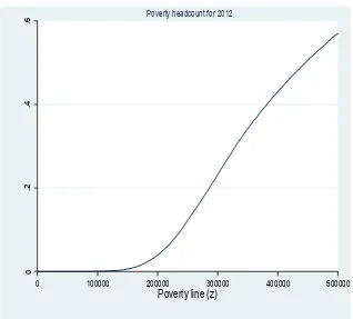
poverty headcount differences are statistically significant throughout the poverty lines between IDR.40,000 and IDR.200,000. The findings clearly show that the larger the poverty line, the greater the difference between the headcounts of the two years, which implies that in 2012, for larger poverty lines, the poverty head-count was systematically lower than in 2002.
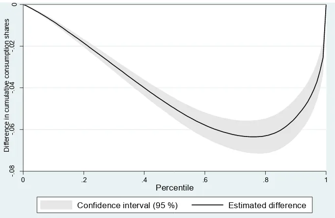
Figure 5. Difference Between 2012 and 2002 Lorenz Curves shows the difference between the 2012 and the 2002 Lorenz curves (and the associated 95 percent confidence intervals). It is evident from the graph that inequality deteriorated significantly between 2002 and 2012. In 2012, the bottom 20 percent of the Indonesian population enjoyed around eight percent of total consumption, while the top 20 percent was responsible for around 47 percent. The bottom 20 percent of the population lost approximately 1.5 percent of total national consumption between 2002 and 2012 (a 15 percent decrease in their respective share), while the top 20 percent of the population has seen its share in total consumption rise by six percent in just ten years (a 15 percent increase in their respective share).
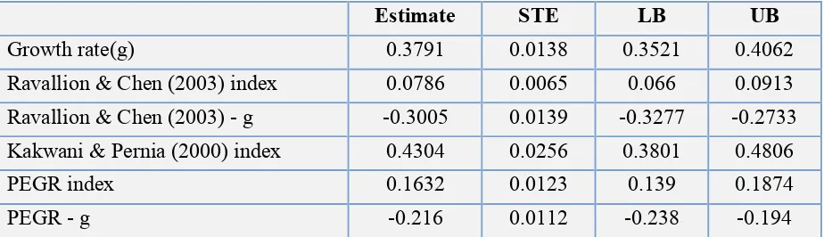
Table 5. Pro-Poor Indices for Indonesia, 2002-2012 provides estimates and confidence intervals for Indonesia’s 2002-2012 growth rate (denoted by the variable - g), and also for the three different pro-poor indices: Ravallion and Chen (2003) index, Kakwani, Khandker and Son (2003) - poverty-equivalent growth (PEGR) rate index, and the Kakwani and Pernia (2000) index. All of the three indices of absolute pro-poorness are statistically greater than zero; this means that the change from 2002 to 2012 has decreased absolute poverty. The Ravallion and Chen-PPG >0, and the changes during 2002-2012 are absolutely pro-poor, but
have first order dominance over the initial distribution. However, since the PPG index is less than the growth rate of the mean population income, growth during the 2002-2012 period cannot be deemed relatively pro-poor, as the distributional shifts have gone against the poor. The PEGR index is greater than zero, but less than mean growth in population income, and thus characterises a ‘trickle-down’ situation (Kakwani, Khandker, and Son (2003)) in which the poor have received proportionately less benefit from growth than the non-poor. So it is clearly evident from the PEGR that over the 2002-2012 period, growth reduced poverty, but has been accompanied by increasing inequality. Alternatively, it can be seen that the estimates of Ravallion and Chen (2003) PPG-index minus g and of Kakwani, Khandker and Son (2003) PEGR-index minus g are all negative, indicating that growth has not been
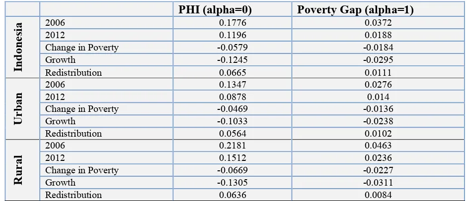
relatively pro-poor. Thus it can be inferred that the growth rates of the incomes of the poor have not been high enough to follow the growth rate in average income, and their relative shares in total consumption have decreased during the 2002-2012 period. Similarly, during the 2006-2012 period, all pro-poor indices display the same growth trend, with the distributional shifts working against the poor (Table A2. Pro-Poor Indices for Indonesia, 2006-2012).
the 10th percentile has increased only by around ten percent (average annual increase of one percent), whereas consumption at the 90th percentile had a 50 percent increase (average annual increase of five percent) during the 2002-2012 period. The slope of the growth incidence curve, and specifically its steepness and upward direction, imply that in general growth has been accompanied by rise in inequality over the 2002-2012 period due the rate of income growth of individuals in the upper income percentiles being higher than the income growth rate of the poor.
Additionally, the proportional changes3 relative to the growth rate in mean consumption also vary significantly across percentiles. As reported in Table 5. Pro-Poor Indices for Indonesia, 2002-2012, the mean growth in consumption is around 38 percent, which evidently exceeds the growth rates experienced by most Indonesians. Except for the top quintile, households in the bottom four quintiles experienced below average growth rates of consumption. This evidence of inequality levels increasing substantially between 2002 and 2012 is also consistent with the fact that growth rates have not been roughly proportional across percentiles.
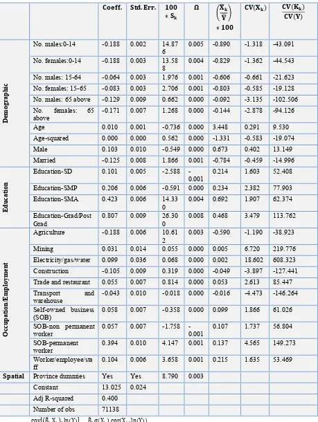
Table 6. Regression-based Inequality Decompositions – 2012 and Table 7. Regression-based Inequality Decompositions – 2002 provide the semi-log regression results and quantify the importance of various factors that have contributed to total in inequality in Indonesia during the 2002-2012-time period. The first column of each table gives the coefficients from a linear expenditure equation estimated by Ordinary Least Squares (OLS) on the full sample of households, while the second column gives standard errors. All estimated coefficients are highly statistically significant with the expected signs. The tables show that per-capita expenditures decrease with number of household members and increase with age. The tables also show that expenditures are higher for urban and non-agricultural households, and that education raises expenditures, increasingly so for higher levels of education.
Next, the inequality decomposition results answers the two questions of Fields (1998) and Morduch and Sicular (2002) in their proposed decomposition methodologies. First, given an expenditure generating function estimated by a standard semi-logarithmic regression, how much consumption inequality is accounted for by each explanatory factor? Second, how much of the difference in income inequality between one date and another is accounted for by education, by potential employment characteristics, and by the other explanatory factors? In
particular, policy makers would like to know whether observed changes in inequality between two periods of time are due to changes in the returns to factors (e.g. education) or to changes in the distribution of factors of production (for example due to changes in demographic characteristics).
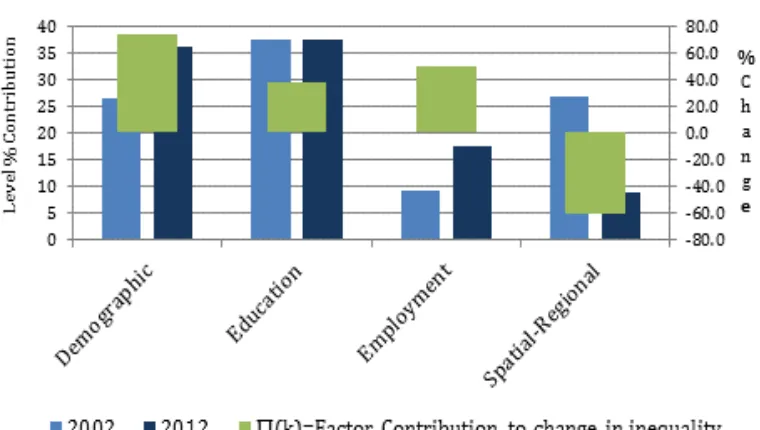
Figure 6. Growth Incidence Curve and column 3 of Tables 6. Regression-based inequality decompositions – 2012 and Table 7. Regression-based Inequality Decompositions – 2002 answers the above questions and summarises the overall group (demographic, education, employment and spatial-regional characteristics) contributions to total inequality for 2002 and 2012. It is clearly evident that differences in education, demographics, geographic location and employment have contributed significantly to total inequality. However, the differentials in expenditure by education level have been relatively larger than for other factors. Theoretically, higher education inequality should be associated with higher income inequality, as a higher educational level should duly ensure a higher income. Thus, differences in educational achievements imply differences in the ability to earn income and consequently disparities in expenditure. During both 2002 and 2012, education differences in expenditure have contributed substantially (37 percent on average) to overall inequality, suggesting that education policies have substantially more redistributive impacts. It is also important to note that primary education has an equalising effect on poverty. This is understandable, since those who are poor are most often educated only up to primary level. To enhance this welfare equalising effect, policy initiatives are needed to increase the returns and attainment of primary education among the poor.
For both 2002 and 2012, demographic characteristics (household size and dependency ratio) were the most important variables after education, with an average factor inequality weight of around 27 percent in 2002 and later rising to 36 percent in 2012. As expenditure inequality is mostly measured on the basis of the average expenditure of the household members, the composition of a household has an impact on income inequality. It has been presumed that the less homogeneous4 the household, the higher the consumption inequality, because the households of different types have different incomes and expenditures per household member (Wilkie, 1996). It is not difficult to infer that poor households have a higher dependency ratio (or lower per capita labour input) and thus a lower level of consumption. Usually, the birth rate is higher among the families at the bottom of the distribution, making the consumption
4
per family member even smaller in this group of population, and increasing the overall inequality. Substantial welfare gaps also exist between households from different regions and whose members are engaged in different employment activities. These gaps are more visible for employment in 2012 and for geographic locations in 2002. Formal sector workers fared better in terms of wellbeing than informal sector employees and consequently, contribute positively to measured income inequality.
5. Conclusions and Policy Implications
In this study, we have examined poverty, inequality and pro-poor changes in Indonesia from 2002 to 2012. During this period, the ordinary growth rate of a household’s income per capita was 38 percent. The growth rate varied from ten percent (with an average annual increase of one percent) for the poorest decile to 50 percent (average annual increase of five percent) for the richest decile, while the rate of pro-poor growth was around 13-15 percent throughout. All poverty indicators suggest that economic growth in Indonesia was particularly beneficial for those located at the top of the distribution. Indeed, for all the three pro-poor indices and estimated GICs, we find that the only positions that grew more than the mean where those above the top most quintiles, which suggests that the gains from growth were highly concentrated at the top of the income distribution. Indonesia’s growth benefitted mainly to the relatively rich households; the poor gained little and often lost from it. Success achieved in macroeconomic management, strong domestic demand, growth in working-age population, consumer class and private investment have apparently not given Indonesian households living near and below the poverty line enough productive employment and economic opportunities to decrease their relative deprivation, nor have they fostered a more inclusive society.
Regression-based decompositions also found that education differences in expenditure to have contributed substantially (37 percent on average) to overall inequality, suggesting that education policies have substantially more redistributive impacts. Decompositions for the change in inequality during the 2002-2012 period shows that the largest contribution to Indonesia’s rising inequality stems from demographic and employment factors. Most of the inequality widening effects that stemmed from these factors has been offset to a certain extent by the narrowing disparities among households by spatial and regional characteristics. Market reforms, unleashed trade activities, increased factor mobility and successful attempts by the Indonesian government to direct resources to the poorer regions can be identified as sources of this equalising spatial effect over time. This finding also justifies regional development programmes and campaigns.
policy options need to give increasingly more weight to alleviating the effect of rural-urban migration on urban poverty.
Therefore, better social integration of rural migrants through better-functioning and more open labour markets will help minimise the adverse impacts of rural-urban migration. Rural migrants’ needs to be provided with market-relevant education and vocational training that would enable them to participate in labour markets and partake in the fruits of urban growth, without excluding them socially and widening the gap in urban inequality. Furthermore, since rural-to-urban migrants are usually engaged in informal employment, policies aimed at integrating and linking informal labour with the formal sector will render growth more pro-poor and inclusive.
With regard to gender, policies that encourage the participation of women in education and in the labour force can produce substantial differences in the distribution of family income and welfare. Empowering women can be one of the most effective ways of increasing household welfare and community empowerment. Investing in female education and employment will further increase the labour force for production and economic growth. It will also indirectly aid pro-poor economic growth, for an instance by lowering fertility and population growth rates and improving the health and education of the next generation5.
Other pro-poor policies include improving access to credit and minimising credit market failures. This will enable poor households to engage in productive, income-generating activities and for many would-be entrepreneurs to escape from the poverty trap. Issuing land and property titles will also increase the ability of the poor to obtain credit and make it easier for them to sell or borrow against these assets for emergency income. It is also imperative, the government of Indonesia launch better-targeted and more innovative social transfer programmes aimed at reducing disparities in access to basic education and health. These programmes should assist the poor in acquiring the skills that they need to compete in new and emerging markets. A classic example is Latin America, where it invested in schools and pioneered conditional cash transfers for the very poor, and is now the only region where inequality in most countries has fallen.
In essence, policies increasing school enrolment and achievement, effective family planning programmes that reduce the birth rate and dependency load within poor households, programmes facilitating urban-rural migration and labour mobility, infrastructure connecting leading and lagging regions, and policies granting priorities for specific social groups (such as children, elderly, illiterate, informal workers and agricultural households) in targeted interventions will serve to simultaneously stem rising inequality and accelerate the pace of economic growth and poverty reduction in Indonesia.
References
Atkinson, A.B. (1987), On the Measurement of Poverty, Econometrica 55, 749–764.
Bhagwati, J.N. (1988), Poverty and Public Policy, World Development Report, Vol. 16 (5), 539-654.
Banerjee, A. V. and E. Duflo (2005), Growth Theory through the Lens of Development Economics, Amsterdam: North Holland, vol. 1A, 473–552.
Coudouel A., Dani A.A. and Paternostro S. (2006), Poverty and social impact analysis of reforms: lessons and Examples from Implementation. World Bank. Washington D.C.
Datt, G., and M. Ravallion (1992), Growth and Redistribution Components of Changes in Poverty Measures: A Decomposition with Applications to Brazil and India in the 1980s. Journal of Development Economics 38 (2), 275–295.
Freidman, Jed. (2002), “How Responsive is Poverty to Growth? A Regional Analysis of Poverty, Inequality, and Growth in Indonesia, 1984-1999.” RAND Working Paper, June. Foster, J., Shorrocks, A.F., (1988). Poverty orderings. Econometrica 56, 173–177.
Heltberg, R. (2001), “The poverty elasticity of growth” Institute of Economics, University of Copenhagen, Unpublished manuscript.
Jain, L.R. and Tendulkar, S.D. (1990), 'The Role of Growth and Redistribution in the Observed Change in Head-count Ratio Measure of Poverty: A Decomposition Exercise for India', IndianEconomic Review, XXV, 165-205.
Kakwani, N (1993), Poverty and Economic Growth with Application to Côte d’Ivoire,
Review of Income and Wealth, 39(2), 121–39.
Kakwani, N. (1997), 'On Measuring Growth and Inequality Components of Poverty with Applications to Thailand', Discussion Paper, School of Economics, The University of New South Wales, Australia.
Kakwani, N., S. Khandker, and H. Son (2003), Poverty Equivalent Growth Rate: With Applications to Korea and Thailand, Technical Report, Economic Commission for Africa. Kakwani, N. and Pernia, E. (2000), What is Pro-poor Growth, Asian Development Review, Vol. 16, No.1, 1-22.
Kakwani, N. and Son, H. H. (2008), Poverty Equivalent Growth Rate," Review of Income and Wealth, Vol. 54, No. 4, pp. 643-655.
Morduch, J. and Sicular, T. (2002), “Rethinking inequality decomposition, with evidence from rural China”, The Economic Journal, vol. 112, pp. 93-106.
Ravallion, M. (2004a), Growth, Inequality, and Poverty: Looking Beyond Averages, Oxford: Oxford University Press, chap. 3, UNU-WIDER studies in development economics.
Ravallion, M. and Chen, S. (2003), Measuring Pro-poor Growth, Economic Letters, Vol. 78 (1), 93-99.
Ravallion, M., Huppi, M., (1991), Measuring changes in poverty: a methodological case study of Indonesia during an adjustment period. World Bank Economic Review 5, 57–84. Said, A., W. Widyanti (2002), The Impact of Economic Crisis on Poverty and Inequality. In Khandker, S (Ed.). The impact of the East Asian Financial Crisis Revisited. World Bank Institute (WBI) and the Philippine for Development Studies (PIDS).
Shorrocks, A. F. (1999), 'Decomposition Procedures for Distributional Analysis: A Unified Framework Based on the Shapley Value', mimeo.
Sumarto, S., Suryahadi, A and Widyanti, W., (2005), Assessing the Impact of Indonesian Social Safety Net Programmes on Household Welfare and Poverty Dynamics‟, The European Journal of Development Research, Vol.17, No.1, March 2005, pp.155–177
Sumarto, S. and Bazzi, S., (2011), Social Protection in Indonesia: Past Experiences and Sectoral Components of Economic Growth on Poverty: Evidence from Indonesia”, Journal of Development Economics, 89(1), pp. 109-117.
Suryahadi, A., Hadiwidjaja, G., Sumarto, S. (2012), Economic growth and poverty reduction in Indonesia before and after the Asian financial crisis. Bulletin of Indonesian Econommic Studies, 48(02), pp. 209-227.
Timmer, P. (2004), The Road to Pro-poor Growth: Indonesia's experience in regional perspective. Bulletin of Indonesian Economic Studies, 40(2), 177-207.
Figure 1. Annualised Change in Inequality of Expenditure or Income – 1990s and 2000s
Source: PovcalNet and ADB (2012)
Figure 2. Number and Percentage of Poor People in Indonesia
Figure 3. Gini and Expenditure Shares
Source: Susenas and BPS Data, various years
Figure 4a. FGT Curve (alpha=0)
Source: Susenas and BPS Data, various years
0
.2
.4
.6
0 100000 200000 300000 400000 500000
Poverty line (z)
FGT Curve (alpha=0)
Figure 4b. Difference between FGT Curves (alpha=0)
Source: Susenas and BPS Data, various years
Figure 6. Growth Incidence Curve
Source: Susenas and BPS Data, various years
Figure 7. Regression-based Inequality Decompositions
Source: Susenas and BPS Data, various years Growth rate in mean
0
.2
.4
.6
0 .18 .36 .54 .72 .9
Percentiles (p)
Confidence interval (95 %) Estimated difference Indonesia, 2002-2012
Table 1. Regional Poverty and Inequality
Source: Data form ADB inclusive growth indicators and PovcalNet
Poverty
incidence
(PPP $2 - per
day)
Income Share
- Lowest
Quintile
Income share
- Highest
Quintile
Ratio of
Highest
Quintile to
Lowest
Quintile
China 29.8 5.0 47.9 9.6
Cambodia 53.3 7.5 45.9 6.1
Indonesia 46.1 8.3 42.8 5.1
Lao PDR 66.0 7.6 44.8 5.9
Malaysia 2.3 4.5 51.5 11.3
Philippines 41.5 6.0 49.7 8.3
Thailand 4.6 6.7 47.2 7.1
Table 2. Regional Socio-Economic Indicators: Regional Socio-Economic Indicators
Province GDP-Share-2011 Gini-2012 Poverty-2012 HDI-2011
Aceh 1.42 0.32 19.50 72.16
Kepulauan Bangka Belitung 0.50 0.29 5.50 73.37
Table 3. Profile of Poverty and Inequality, 2002-2012: Profile of Poverty and Inequality, 2002-2012
Table 4. Growth – Redistribution Decompositions, Indonesia 2002-2012
PHI (alpha=0) Poverty Gap (alpha=1)
Change in Poverty -0.0619 -0.0120 Growth -0.1757 -0.0412
Change in Poverty -0.0569 -0.0105 Growth -0.1511 -0.0339 Change in Poverty -0.0597 -0.0123
Table 5. Pro-Poor Indices for Indonesia, 2002-2012
Estimate STE LB UB
Growth rate(g) 0.3791 0.0138 0.3521 0.4062 Ravallion & Chen (2003) index 0.0786 0.0065 0.066 0.0913 Ravallion & Chen (2003) - g -0.3005 0.0139 -0.3277 -0.2733 Kakwani & Pernia (2000) index 0.4304 0.0256 0.3801 0.4806 PEGR index 0.1632 0.0123 0.139 0.1874 PEGR - g -0.216 0.0112 -0.238 -0.194
Table 6. Regression-based Inequality Decompositions – 2012
No. females:0-14 -0.188 0.003 13.58 8
Electricity/gas/water 0.099 0.036 0.068 0.000 0.002 18.602 608.323
𝐂𝐨𝐞𝐟𝐟. 𝐒𝐭𝐝.𝐄𝐫𝐫. 𝟏𝟎𝟎
Electricity/gas/water -0.019 0.096 -0.007 0.000 0.000 -23.113 -809.133
Table A1. Growth – Redistribution Decompositions, Indonesia 2006-2012
Table A2. Pro-Poor Indices for Indonesia, 2006-2012
Estimate STE LB UB
STD: standard error, LB: lower bound of 95% confidence interval, UB: upper bound of 95% confidence interval
PHI (alpha=0) Poverty Gap (alpha=1)
Change in Poverty -0.0579 -0.0184
Growth -0.1245 -0.0295
Change in Poverty -0.0469 -0.0136
Growth -0.1033 -0.0238
Change in Poverty -0.0669 -0.0227
Growth -0.1305 -0.0311