AN AUTOMATIC FILTER ALGORITHM FOR DENSE IMAGE MATCHING POINT
CLOUDS
DONG YouQiang a,b, ZHANG Li b, CUI XiMin a, *, AI HaiBinb
a College of Geoscience and Surveying Engineering, China University of Mining and Technology(Bei Jing), Beijing 100083, China-
[email protected], cxm @cumtb.edu.cn
b Chinese Academy of Surveying and Mapping, Beijing 100830,China-(Zhangl, ahb)@casm.ac.cn
KEY WORDS: Filtering, Dense Image Matching Point Clouds, Density, Angles, TIN
ABSTRACT:
Although many filter algorithms have been presented over past decades, these algorithms are usually designed for the Lidar point clouds and can’t separate the ground points from the DIM (dense image matching, DIM) point clouds derived from the oblique aerial images owing to the high density and variation of the DIM point clouds completely. To solve this problem, a new automatic filter algorithm is developed on the basis of adaptive TIN models. At first, the differences between Lidar and DIM point clouds which influence the filtering results are analysed in this paper. To avoid the influences of the plants which can’t be penetrated by the DIM point clouds in the searching seed pointes process, the algorithm makes use of the facades of buildings to get ground points located on the roads as seed points and construct the initial TIN. Then a new densification strategy is applied to deal with the problem that the densification thresholds do not change as described in other methods in each iterative process. Finally, we use the DIM point clouds located in Potsdam produced by Photo-Scan to evaluate the method proposed in this paper. The experiment results show that the method proposed in this paper can not only separate the ground points from the DIM point clouds completely but also obtain the better filter results compared with TerraSolid.
1. INTRODUCTION
With the development of new pixel-wise matching algorithms and the improvement in camera technology, the dense, reliable and accurate 3D DIM point clouds have been generated by research groups and commercial vendors and have been used in many fields, such as land cover classification(Rau et al., 2015), 3D-building modelling(Dahlke et al., 2015; Maltezos and Ioannidis, 2015) and digital terrain modelling(Li and Gruen, 2004). In these applications, point clouds filtering is still an essential step. Although the DIM point clouds may reach the high accuracy and resolution corresponding to the GSD (ground sampling distance, GSD) of the original images for rather complex urban environments(Haala and Cavegn, 2016; Remondino et al., 2014), there are still many differences between the DIM and Lidar point clouds. Some works(Rau et al., 2015; Themistocleous et al., 2016) have pointed that the differences contain the point density, variation. In fact, besides these discrepancies above, the DIM point clouds don’t have scan line, echo times and intensity information either compared with Lidar point clouds. Whether these differences will affect the filter results has not been discussed in previous works.
In the extraction of bare earth, some researchers(Gerke and Xiao, 2014; Maltezos and Ioannidis, 2015; Nex and Remondino, 2012) choose the lowest point inside a window of a certain size varies depending on the scene so as to avoid false ground detection. And a densification process via meshing and resampling with an appropriate point density is carried out. Construct DSM using the ground points. The height difference between the point need to be processed and the closest ground point is computed. If the height difference is lower than the threshold, the point is regarded as the ground point, otherwise, the point is an off-ground point. In these applications, the researchers often pay more attention on the extraction of the off-ground points, the thresholds will reach
* Corresponding author
2~4m. The remaining ground points still contain many small objects.
From this brief overview above, we can conclude that in the filtering process, the DIM point clouds are usually rarefied firstly and then are handled using the filter algorithms designed for Lidar point clouds(Axelsson, 2000; Sithole and Vosselman, 2004). This filtering way on the one hand will cause the absence of the terrain features, on the other hand can’t extract the whole ground points completely. To avoid these drawbacks, making use of the original DIM point clouds directly to extract the ground points is necessary.
In this paper, a new filter algorithm aimed at DIM point clouds is developed on the basis of Axelsson. Due that the main advantage of DIM point clouds is the visibility of facades of buildings, the proposed algorithm is mainly for the urban areas. Compared to the methods mentioned above, the main contributions of this paper are summarized as follows:
The differences between Lidar and DIM point clouds which influence the filter results are discussed. Here we focus on the effect produced by the differences on the filter results;
A filter method aimed at DIM point clouds is presented. Using the method, the ground points can be extracted from the DIM point clouds completely.
2. THE DIFFERENCES BETWEEN LIDAR AND DIM POINT CLOUDS
The major goal of this section is to present the differences between DIM and Lidar point clouds. This section is divided into two parts. In the section 2.1, we will introduce the data sources used in this paper. Section 2.2 introduces the differences between the DIM and Lidar point clouds and analyses the impact produced by the differences on the filtering.
2.1 Data Sources
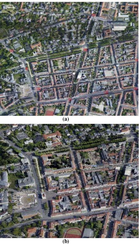
In this paper, the data set are collected from Trimble AOS system on September 17 in 2012 in Potsdam, Germany. This system is composed of three AOS cameras with a 49*37mm2 sensor size and a . �� pixel size, which can capture 7228*5428 pixels. At each exposure time, it acquires one vertical image (with a �� focal length) and 2 oblique images (with a �� focal length) that point in four opposing directions with tilt angles at approximately 30° to 40°.Then the cameras rotate 90 degree, and exposure. Thus, one point observed by the two oblique images from opposing directions will construct an intersection angle at 0° − 0°.The flying height above ground is approximately 0� and the ground sampling distance (GSD) for all cameras is approximately 10cm.
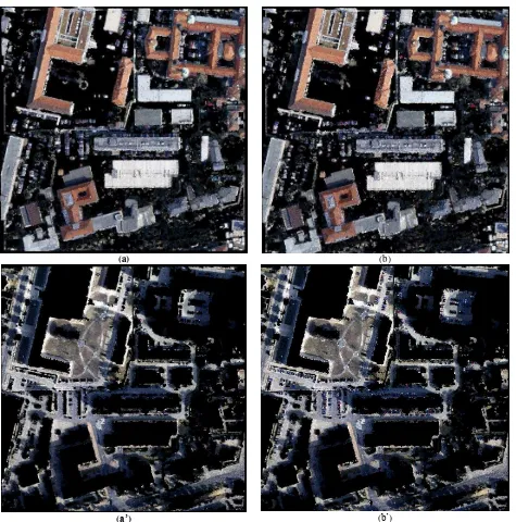
(a)
(b)
Figure 1. The DIM point cloud produced using PhotoScan (a).the orthophoto of interesting region (b) the DIM point clouds
210 images(70 VAIs and 140 OAIs ) acquired were used to generate dense point cloud by the commercial software
Photo-Scan Professional(64 bit) and 298113024 points with spectral information were produced and the point density is 34.9/m2. Nine plane regions located on the road (in figure 1(a)) are selected to calculate the variation. The results can be seen in table1.
Region The
Table1. The deviation values for all the selected plane regions
2.2 The differences between Lidar and DIM point clouds
Although the differences between Lidar and DIM point clouds have been discussed in some works, we pay more attention on the differences which affect the filter results here. In addition to the density and variation, echo intensity and times information, scan line and penetrability also affect the filter results. The comparison results can be seen in Table2.
Table 2.the comparison results of Lidar and DIM point clouds
Now we will discuss how these differences above will affect the filtering when we apply the algorithms mentioned in Sithole and Vosselman (Sithole and Vosselman, 2004) to extract the ground points.
2.2.1 Density and variation
vegetation should be removed. According to this, the algorithms designed for the Lidar point clouds aren’t suitable for the DIM point clouds.
2.2.3 Scan line
Usually, the Lidar points arrange along the scan line. This help the data although some algorithm. For example, in Axelsson the initial thresholds are collected in the form of discrete histograms of surface normal angles and elevation difference along the scan line. If we apply the method proposed by Axelsson, it is a problem how to calculate the initial thresholds.
2.2.4 Echo times and intensity
In 1999, Ackermann (Ackermann, 1999) have pointed that the data fusion for the purpose of filtering is necessary. Additional data could be used to further improve the filter algorithms. In terms of Lidar point clouds, both echo times and intensity can be used to improve the filter results. Brovelli(Brovelli et al., 2002) made use of both the first and last pulse data to filter.
2.2.5 Spectral information and the building facades Although the DIM point clouds don’t have scan line, echo times and intensity information, the DIM point clouds contain the spectral information. Besides this, the DIM point clouds produced by the oblique aerial images can detect the building facades. These additional data can help us to filter.
From what has been discussed above, we can conclude that the differences between Lidar and DIM point clouds will affect the filter results from all aspects. In Sithole and Vosselman (Sithole and Vosselman, 2004), the Axelsson can get good filter results for Lidar point clouds. Now we analyse the problems may encounter in filtering of DIM point clouds using the Axelsson.
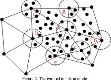
In Axelsson, the algorithm selects the lowest point belong to a user-defined grid as the seed point and constructs a TIN using the seed points. Calculate the distance to the TIN facets and angels to the node and add the point to the TIN if below threshold values. In each iteration, the thresholds will become smaller than the previous iteration. However, the density and variation of DIM point clouds are very high. When the points construct the TIN is enough dense, the angle will become large due to the high variation which leads the points which are ground points in fact can be omitted (see in Figure 2 ).
Figure 2. The ignored points in circles
Besides these, the DIM points don’t have the scan line, the statistics can’t be collected along the scan line. Because the DIM points can’t penetrate the vegetation points aren’t be. If we still choose a lowest point in a user-defined grid, the point may be a vegetation point. If we still adopt the iteration strategy to extract the terrain, good results will not be obtained. The new method must solve these problem. The method proposed is variant on the densification filter developed by Axelsson. This method is aimed at the urban areas.
3. THE METHODOLOGY
As the method in this paper proposed is variant on the densification filter developed by Axelsson, this section consists of selecting seed points, densification of TIN and parameter estimation.
3.1 Selecting seed points
As is described above, the lowest point can’t be the seed points because of the absence of the penetration through the vegetation. Urban areas are consist of roads, buildings, plants and others and seed points should be located on the roads. In other words, a point belong to road is a seed point. The problem on how to select seed points is converted to the problem on how to search road points. Generally speaking, road points are on the side of the building façades can be easily detected using point clouds. Based on this, we can select seed points as below:
step1. Remove the plants
Although NDVI (Normalized Difference Vegetation Index) is a very efficient tool for the detection of plants, some multi-camera systems do not have the near infrared band. In order to expand the application of the algorithm, we use vegetation colour index to remove plants. In this paper, test four vegetation colour indexes(Meyer and Neto, 2008) - NGRDI (normalized green-red difference index, NGRDI), ExG (excess green index, ExG), ExG-ExR (the excess green minus excess red index, ExG-ExR) and GLI (green leafy index, GLI) - are used to eliminate the plants. Compared with the NDVI, the vegetation colour indexes are influenced by the urban environment. By comparison, we choose the GLI to wipe off the plants. whole survey region into regular grids. It is obvious that DoPP value of a grid which contains the building façades is much higher than other grids. We can create a density image according to the DoPP value. If the DoPP value of a grid is beyond the threshold, the corresponding image intensity value is 0; otherwise, the corresponding intensity value is 255.
Figure 3. Choose the seed points
Step4. Constrain the seed points
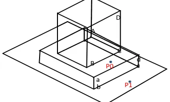
Some seed points selected above in fact may not be on the ground because of the structures of some buildings. As is shown in Figure 4, the point 0 is located on the pedestal of a building. When we search seed points along a line produced by the projection of the facades onto the horizontal plane, the point 0 will be taken for a seed point. The wrong points are usually are near the true seed points. To delete the errors, search the neighbourhood of every seed point. If a
Figure 4. The locations of alternative seed points to be deleted
3.2 Densification Process
In section 3.1, the seed points have been selected. Calculate the initial densification thresholds include the distance and angle firstly and add the points below the thresholds to the initial TIN constructed by seed points. Now, the densification starts. As is described in section 2.2, when the density of TIN is denser, the distance threshold from a point to the facet becomes smaller and the angle threshold may increase. The density changes, the thresholds change. In fact, a density value corresponds to a pair of thresholds. The practice proves that the interpolation accuracy using regular triangular is higher compared with al-long-narrow triangular. To get the better results and calculate the threshold fast, the points are divided into regular grids according to the specified density. In the iterative process, the density of the TIN changes from low to high. The iterative process can be described as:
(1) Specify the density of the TIN.
(2) Calculate parameters using the points have been added to ground at a specified density.
(3) Add the points to the ground at the specified density. To add as many points as possible, we will construct several TINs at the specified density. Add a point to ground point dataset if the point below threshold values.
(4)Increase the density to a specified value. Continue (1) to (3) until all the points are classified as ground or object.
3.3 Parameter Estimation
3.3.1 The threshold of GLI
In this paper, GLI are used to extract the vegetation points. The thresholds of the remaining colour indices can be determined by OSTU.
3.3.2 The threshold of facades of buildings
We project the whole points on the grid net. The threshold of facades of building is the number of total points in a grid size. In the process of searching the seed points, we suppose that the density of DIM point clouds is DEN, the size of the grid is GRIDESIZE. Thee default height of the building is H. If the matching result of ground is in line with the facades, the
number of points belong to a grid containing the façade can be described as:
DEN* h*GRIDESIZE+GRIDESIZE*GRIDESIZE (3)
However, the facades usually contain the glass texture. To get accurate threshold, we need multiply by a coefficient. When the projection density beyond the value, it is believed that this point is located on the edge of the building.
3.3.3 The threshold of the densification of TIN
Axelsson can’t collect statistics from the points produced by the oblique images because of the absence of the scan line. Fortunately, the existence of building facades can provide the clue of searching initial densification parameter.
(a) (b)
Figure 5. Estimate the initial thresholds
As is shown in Figure 5(a), triangle is a facet of the TIN constructed by the seed points obtained in section 3.1 and point is on the ground. The distance from the point to the facet is usually small. When the point is on the façade of a building as is shown in Figure5 (b), the distance will sharply become big. The trend line can be seen in Figure6. The distance threshold is located in the red ellipse and we can get distance threshold by the Twi-difference of distances.
Figure 6. The left: Accumulated histogram for distances; the right Accumulated histogram for Twi-differences of distances
3.3.4 The densification thresholds
To estimate the densification parameters, choose a point in each grid and construct the TIN at the specified density. If the grid doesn’t contain ground points, skip it. Calculate the angle and distance of every remaining ground point to the TIN. Project the thresholds onto the plane. The x-axis stands for the min angle and the y-axis stands for the distance. The thresholds can be estimated on the plane.
4. EXPERIMENT RESULTS
4.1 The filter results and discussion
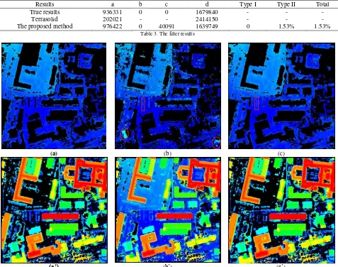
It has been shown that although the ground points are extracted by Terrasolid, a large number of terrain points are omitted in filtering and are regarded as the objects points from the Figure 7(b’). The number of ground and object points after filtering can be seen in Table 3. It is obvious that the number of type I errors produced by the proposed method is less than Terrasolid because of the application of new densification strategy. In terms of reducing type I errors, the proposed method is a complete victory compared with Terrasolid in the DIM point clouds filtering.
Although the number of the ground points extracted by Terrasolid is less than by the proposed method, the percentage of
object points regarded as ground points is larger. Two prominent objects labelled by red ellipsis in Figure 7(b) are categorized as ground. This is caused by the wrong seed points. For the small objects such as cars labelled by rectangles in Figure 7(b) and Figure 7(c), the performances of the two methods are almost the same. The number of the type II error produced by Terrasolid is
larger. Type I error is b *100%
ab
, the type II error is
* 100% c
cd
, the total error is b c * 100% a b c d
.The
percentages of type I and II error in the results of filtering the datasets with two methods are given in table 3.
Results a b c d Type I Type II Total
True results 936331 0 0 1679840 - - -
Terrasolid 202021 - - 2414150 - - -
The proposed method 976422 0 40091 1639749 0 1.53% 1.53%
Table 3. The filter results
(a) (b) (c)
(a’) (b’) (c’)
Figure 7. The filter results: top left: the ground, top middle: the ground extracted by Terrasolid, top right: the ground extracted by the method proposed in this paper; bottom left: the object, bottom middle: the ground extracted by Terrasolid, bottom right: the object extracted by the method proposed in this paper
Compare the filter results with the true classified results. The filter results are the almost same with the true classified results. However, the small objects such as cars are classified as ground or only the top of the cars are classified as objects as is shown in Figure 8. The mainly reason is that the angle threshold become larger with the densification. The joint of cars and ground is smooth transition.
4.2 The densification thresholds
As is shown in section 2.2, the distance threshold will become smaller and the angle threshold will become bigger with the
increase of the density. Table 4 gives the different thresholds at the specified thresholds. From table 4, the change of the thresholds is compatible with the theory described in section 2.2.
density distance
(m)
angle (m)
Initial 0.35 0.058
4m 0.25 0.228
2m 0.22 0.35
5. CONCLUSION
This paper presented a method for automatically filter original DIM point clouds in order to obtain an accurate digital terrain model. The method applies new densification strategy to densify the TIN and add the ground point as many as possible. In the filter process, the density of TIN, the distance threshold and the angle
threshold are estimated. The experiment results show that the method proposed in this paper can obtain digital terrain model. The main error is type II error. Due that the method makes use of the building facades to search seed points and the advantage of the DIM point clouds is visibility of facades, the proposed method is mainly used in urban scenarios.
(a) (b)
(a’) (b’)
Fig. 8 The comparison between true results and the results produced by the proposed method: top left: the true object points; top right: object points extracted by the method proposed in this paper; bottom left: true ground points; bottom right: ground points extracted by the
method proposed in this paper
REFERENCES
Ackermann, F., 1999. Airborne laser scanning—present status and future expectations. Isprs Journal of Photogrammetry & Remote Sensing 54, 64-67.
Axelsson, P., 2000. DEM generation from laser scanner data using adaptive TIN models, International Archives of Photogrammetry & Remote Sensing.
Brovelli, M.A., Cannata, M., Longoni, U.M., 2002. Managing and processing LIDAR data within GRASS.
Gerke, M., Xiao, J., 2014. Fusion of airborne laserscanning point clouds and images for supervised and unsupervised scene classification. ISPRS Journal of Photogrammetry and Remote Sensing 87, 78-92.
Haala, N., Cavegn, S., 2016. High Density Aerial Image Matching: State-Of-the-Art And Future Prospects. ISPRS - International Archives of the Photogrammetry, Remote Sensing and Spatial Information Sciences XLI-B4, 625-630.
Li, Z., Gruen, A., 2004. Automatic DSM generation from linear array imagery data. International Archives of Photogrammetry, Remote Sensing and Spatial Information Sciences XXXV-B3.
Maltezos, E., Ioannidis, C., 2015. Automatic Detection Of Building Points From Lidar And Dense Image Matching Point Clouds. ISPRS Annals of Photogrammetry, Remote Sensing and Spatial Information Sciences II-3/W5, 33-40.
Meyer, G.E., Neto, J.C., 2008. Verification of color vegetation indices for automated crop imaging applications. Computers and Electronics in Agriculture 63, 282-293.
Nex, F., Remondino, F., 2012. Automatic Roof Outlines Reconstruction From Photogrammetric Dsm. ISPRS Annals of Photogrammetry, Remote Sensing and Spatial Information Sciences I-3, 257-262.
Rau, J.Y., Jhan, J.P., Hsu, Y.C., 2015. Analysis of Oblique Aerial Images for Land Cover and Point Cloud Classification in an Urban Environment. Geoscience & Remote Sensing IEEE Transactions on 53, 1304-1319.
Remondino, F., Spera, M.G., Nocerino, E., Menna, F., Nex, F., 2014. State of the art in high density image matching. The Photogrammetric Record 29, 144-166.
Shi, W.Z., Li, B.J., Li, Q.Q., 2005. A method for segmentation of range image captured in vehicle-borne laserscanning based on the Density of Projected Points. Acta Geodaetica Et Cartographic Sinica 34, 95-100.
Sithole, G., Vosselman, G., 2004. Experimental comparison of filter algorithms for bare-Earth extraction from airborne laser scanning point clouds. ISPRS Journal of Photogrammetry and Remote Sensing 59, 85-101.