USING MULTI-SCALE FEATURES FOR THE 3D SEMANTIC LABELING OF
AIRBORNE LASER SCANNING DATA
R. Blomley, M. Weinmann
Institute of Photogrammetry and Remote Sensing, Karlsruhe Institute of Technology (KIT), Englerstr. 7, 76131 Karlsruhe, Germany - (rosmarie.blomley, martin.weinmann)@kit.edu
Commission II, WG II/4
KEY WORDS:3D Semantic Labeling, Airborne Laser Scanning, Point Cloud, Multi-Scale Features, Classification
ABSTRACT:
In this paper, we present a novel framework for the semantic labeling of airborne laser scanning data on a per-point basis. Our framework uses collections of spherical and cylindrical neighborhoods for deriving a multi-scale representation for each point of the point cloud. Additionally, spatial bins are used to approximate the topography of the considered scene and thus obtain normalized heights. As the derived features are related with different units and a different range of values, they are first normalized and then provided as input to a standard Random Forest classifier. To demonstrate the performance of our framework, we present the results achieved on two commonly used benchmark datasets, namely theVaihingen Datasetand theGML Dataset A, and we compare the results to the ones presented in related investigations. The derived results clearly reveal that our framework excells in classifying the different classes in terms of pointwise classification and thus also represents a significant achievement for a subsequent spatial regularization.
1. INTRODUCTION
Automated scene interpretation has become a topic of major in-terest in photogrammetry, remote sensing, and computer vision. Focusing on the analysis of urban areas, data acquisition is mean-while typically performed in terms of acquiring data in the form of sampled point clouds via laser scanning. To reason about spe-cific objects in the scene and use the respective information for modeling or planning processes, many applications rely on a se-mantic labeling of the acquired point clouds as an initial step. Such a semantic labeling is typically achieved via point cloud classification (Chehata et al., 2009; Shapovalov et al., 2010; Mal-let et al., 2011; Niemeyer et al., 2014; Hackel et al., 2016; Wein-mann, 2016; Grilli et al., 2017), where the objective is to assign a semantic label to each point of the point cloud.
To foster research on the automated analysis of large urban ar-eas acquired via airborne laser scanning and thus represented in the form of point clouds, theISPRS Benchmark on 3D Seman-tic Labeling(Rottensteiner et al., 2012; Cramer, 2010) has been released. However, only few approaches have been evaluated on the provided dataset so far (Niemeyer et al., 2014; Blomley et al., 2016a; Steinsiek et al., 2017), and correctly classifying the dataset turned out to be rather challenging as several classes re-veal a quite similar geometric behavior (e.g. the classesLow Veg-etation, Fence/HedgeandShrub), while others combine sub-groups of different appearance (e.g. the classRoof, which com-bines both pitched and terrace roofs) as indicated in Figure 1. In this paper, we focus on the classification of airborne laser scan-ning data. We present a novel classification framework using collections of spherical and cylindrical neighborhoods as well as spatial bins as the basis for a multi-scale geometric representation of the surrounding of each point in the point cloud. In contrast to a single-scale representation, this allows describing how the local 3D structure behaves across scales. While the spherical and cylindrical neighborhoods serve for deriving metrical fea-tures and distribution feafea-tures, the spatial bins are exploited in
order to approximate the topography of the considered scene and thus obtain normalized heights. To address the fact that the de-rived features are represented in different units and span a differ-ent range of values, we use a normalization to map each differ-entry of the feature vector onto the interval[0,1]. The normalized feature vectors are provided as input to a Random Forest classifier which establishes the assignment to semantic class labels on a per-point basis. In summary, our main contributions are
• the use of a rich diversity of neighborhoods of different scale, type and entity in order to appropriately describe local point cloud characteristics,
• the use of different feature types extracted from the defined neighborhoods,
• the use of a normalized height feature only considering the heights of objects above ground and removing effects aris-ing from the topography of the scene,
• a performance evaluation on two commonly used bench-mark datasets, and
• new baseline results for theISPRS Benchmark on 3D Se-mantic Labeling.
After briefly summarizing related work (Section 2), we present our framework for classifying airborne laser scanning point clouds in detail (Section 3). To demonstrate our framework’s performance, we provide the results obtained for different bench-mark datasets (Section 4), and we subsequently discuss the de-rived results in detail (Section 5). Finally, we provide concluding remarks as well as suggestions for future work (Section 6).
2. RELATED WORK
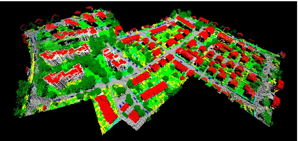
Figure 1. Point cloud colored with respect to nine semantic classes (Roof: red;Fac¸ade: white;Impervious Surfaces: gray;Car: blue; Tree: dark green;Low Vegetation: bright green;Shrub: yellow;Fence/Hedge: cyan;Powerline: black).
2.1 Neighborhood Definition
Many investigations focus on the representation of local point cloud characteristics at a single scale. For such a single-scale rep-resentation, a cylindrical neighborhood (Filin and Pfeifer, 2005) or a spherical neighborhood (Lee and Schenk, 2002; Linsen and Prautzsch, 2001) is commonly used. Thereby, the scale parameter to describe such a neighborhood is represented by either a radius (Filin and Pfeifer, 2005; Lee and Schenk, 2002) or the number of nearest neighbors (Linsen and Prautzsch, 2001). The value of the scale parameter is typically selected heuristically based on knowledge about the scene and data. To automatically select a suitable value in a data-driven approach, it has for instance been proposed to select the optimal scale parameter for each individual point via dimensionality-based scale selection (Demantk´e et al., 2011), where a highly dominant behavior of one of the dimen-sionality features (i.e. linearity, planarity, and sphericity) is fa-vored. A similar approach has been presented with eigenentropy-based scale selection (Weinmann et al., 2015), where the minimal disorder of 3D points is favored.
In contrast to a representation of local point cloud characteristics at a single scale, a multi-scale representation allows a description of geometric properties at different scales and thereby implicitly accounts for the way in which these properties change across scales. To describe local point cloud characteristics at multiple scales, Niemeyer et al. (2014) and Schmidt et al. (2014) used a collection of cylindrical neighborhoods with infinite extent in the vertical direction and radii of1m,2m,3m and5m, respectively. In addition to these neighborhoods, Blomley et al. (2016a,b) also used a spherical neighborhood of locally-adaptive size for each individual 3D point. Thereby, the local adaptation is achieved via eigenentropy-based scale selection (Weinmann et al., 2015), where the optimal scale parameter is directly related to the min-imal disorder of 3D points within a local neighborhood. In con-trast to these neighborhood types, it has also been proposed to use a multi-scale voxel representation (Hackel et al., 2016) or even different entities in the form of voxels, blocks and pillars (Hu et al., 2013), in the form of points, planar segments and mean shift segments (Xu et al., 2014), or in the form of spatial bins,
planar segments and local neighborhoods (Gevaert et al., 2016). Recently, Yang et al. (2017) considered local point cloud charac-teristics on the basis of points, segments and objects as well as local context for analyzing point clouds.
We argue that cylindrical and spherical neighborhoods have the benefit that they rely only on one scale parameter independent of the local point distribution, but we also advocate that in this case of neighborhoods with fixed scale parameters multiple sizes for both of them should be considered. In addition to the cylindrical neighborhoods proposed by Niemeyer et al. (2014) and Schmidt et al. (2014), we hence also use a collection of spherical neigh-borhoods as proposed by Brodu and Lague (2012) in the scope of an investigation focusing on terrestrial laser scanning data. As we focus on ALS data with a significantly lower point density, we do not consider neighborhoods with radii in the centimeter scale. In-stead, we select the same radii as used by Niemeyer et al. (2014) and Schmidt et al. (2014) for cylindrical neighborhoods. Con-sequently, we consider a collection of spherical neighborhoods with radii of1m,2m,3m and5m, respectively. Moreover, we consider one spherical neighborhood of adaptive size, chosen via eigenentropy-based scale selection (Weinmann et al., 2015).
2.2 Feature Extraction
The defined neighborhoods serve as the basis for feature extrac-tion. Thereby, different feature types may be considered and the considered features are typically concatenated to a feature vector:
• Parametric featuresare defined as the estimated parameters when fitting geometric primitives such as planes, spheres or cylinders to the given data (Vosselman et al., 2004). • Metrical featuresdescribe local point cloud characteristics
• Sampled featuresfocus on a sampling of specific proper-ties within a local neighborhood. In this regard,distribution featuresare typically used which describe local point cloud characteristics by sampling the distribution of a certain met-ric e.g. in the form of histograms (Osada et al., 2002; Rusu et al., 2009; Tombari et al., 2010; Blomley et al., 2016a,b).
As our framework should be applicable for the analysis of gen-eral scenes, we do not want to involve strong assumptions on spe-cific geometric primitives to be present in the considered scene. Consequently, we do not take into account parametric features. Instead, we focus on the use of metrical features and distribution features which are widely but typically separately used for a va-riety of applications.
Furthermore, we take into account that the height above ground can be a useful feature to distinguish between some classes of otherwise identical geometry (e.g. Terraced Roof vs. Impervi-ous Surface). As the scene’s landscape is not necessarily flat, we have to estimate the local topography of the scene in order to derive the normalized height feature. However, instead of an ac-curate ground filtering of lidar data for automatically generating a Digital Terrain Model (DTM) (Mongus and ˇZalik, 2012; Sithole and Vosselman, 2004; Kraus and Pfeifer, 1998), we assume that a rough approximation of the local topography is already sufficient to derive the normalized height of each point.
2.3 Classification
The derived feature vectors are provided as input to a classifier which, after being trained on representative training data, can as-sign the respective class labels. In this regard, the straightforward solution consists in selecting a standard approach for supervised classification, e.g. a Support Vector Machine classifier (Mal-let et al., 2011; Lodha et al., 2006), a Random Forest classifier (Chehata et al., 2009; Guo et al., 2011; Steinsiek et al., 2017), an AdaBoost(-like) classifier (Lodha et al., 2007; Guo et al., 2015) or a Bayesian Discriminant Analysis classifier (Khoshelham and Oude Elberink, 2012). However, as these classifiers treat each point of the point cloud individually, they do not take into account a spatial regularity of the derived labeling, i.e. a visualization of the classified point cloud might reveal a “noisy” behavior.
To enforce spatial regularity, local context information can be taken into account. This means that, instead of treating each point individually by considering only its corresponding feature vector, the feature vectors and labels of neighboring points are taken into account as well. In many cases, such a contextual clas-sification involves a statistical model of context, where particu-lar attention has been paid to the use of a Conditional Random Field (Niemeyer et al., 2014; Schmidt et al., 2014; Steinsiek et al., 2017; Landrieu et al., 2017).
In our work, we focus on standard approaches for supervised clas-sification, as respective classifiers are meanwhile available in nu-merous software tools and rather easy-to-use by non-expert users.
3. METHODOLOGY
Our framework consists of different components. As input, the framework only receives the spatial coordinates of 3D points, while other information such as radiometric data or a Digital Ter-rain Model (DTM) are not considered in the scope of our work as they are not consistently or not at all provided for the commonly
used benchmark datasets. Based on the available spatial informa-tion, our framework uses suitable neighborhoods (Section 3.1) for appropriately describing each 3D point with a feature vec-tor (Section 3.2) which, in turn, is first normalized (Section 3.3) and then classified with a standard classifier trained on represen-tative training data (Section 3.4). The main scientific novelty is given by (1) the use of an advanced multi-scale neighborhood and (2) the use of normalized height features.
3.1 Neighborhood Definition
To appropriately describe local point cloud characteristics, we fo-cus on a consideration on point-level and the use of multi-scale neighborhoods as motivated in (Niemeyer et al., 2014; Brodu and Lague, 2012; Blomley et al., 2016a,b). To derive suitable neigh-borhoods serving as the basis for feature extraction, we follow the strategy of selecting multiple neighborhoods of different scale and type (Blomley et al., 2016a,b). In contrast to existing work, we use a rich diversity of neighborhoods to obtain a better de-scription of local point cloud characteristics, and we also consider a neighborhood at a different entity represented by spatial bins:
• As proposed by Niemeyer et al. (2014), we consider a collection of four cylindrical neighborhoods (Ncyl), which
(1) are aligned along the vertical direction, (2) have infinite extent in the vertical direction and (3) have a radius of1m, 2m,3m and5m, respectively.
• As cylindrical neighborhoods with infinite extent in the ver-tical direction do not take into account that points at different height levels might belong to different classes, we also con-sider a collection of five spherical neighborhoods (Nsph).
Four of them have a radius of1m,2m,3m and5m, which is in analogy to the used cylindrical neighborhoods. In addi-tion, we use a spherical neighborhood relying on thek near-est neighbors (Nsph,kopt), whereby the optimal value fork is selected for each 3D point individually via eigenentropy-based scale selection (Weinmann et al., 2015).
• In addition to cylindrical and spherical neighborhoods, we consider spatial bins as the basis for approximating the to-pography of the considered scene. This neighborhood type is derived by partitioning the scene with respect to a horizon-tally oriented plane into quadratic bins with a side length of 20m. In contrast to the other neighborhoods, this neighbor-hood is only used to derive normalized height features.
Thus,10different neighborhoods are used as the basis for feature extraction, and our framework allows for both a separate and a combined consideration of the different neighborhoods.
3.2 Feature Extraction
In our framework, we use geometric features that can be catego-rized with respect to four different feature types:
• Thecovariance features are derived from the normalized eigenvalues of the 3D structure tensor calculated from the 3D coordinates of all points within the considered cylin-drical or spherical neighborhood. These features are given by linearity, planarity, sphericity, omnivariance, anisotropy, eigenentropy, sum of eigenvalues and change of curvature (West et al., 2004; Pauly et al., 2003).
within the considered cylindrical or spherical neighborhood. The respective features are represented by the local point density, the verticality, and the maximum difference as well as the standard deviation of the height values corresponding to those points within the local neighborhood. For the spher-ical neighborhood determined via eigenentropy-based scale selection (Nsph,kopt), the radius of the local neighborhood is considered as an additional feature.
• Theshape distributionshave originally been proposed to de-scribe the shape of complete objects (Osada et al., 2002) and later been adapted to describe characteristics within a cylin-drical or spherical neighborhood (Blomley et al., 2016a,b). Generally, shape distributions are histograms of shape val-ues, which may be derived from random point samples by applying (distance or angular) metrics such as the an-gle between any three random points (A3), the distance of one random point from the centroid of all points within the neighborhood (D1), the distance between two random points (D2), the square root of the area spanned by a trian-gle between three random points (D3) or the cubic root of the volume spanned by a tetrahedron between four random points (D4). For each of these metrics, we randomly se-lect255minimal point samples from the considered neigh-borhood, evaluate the respective metric for each point sam-ple and finally consider the distribution of histogram counts. Thereby, we use histograms consisting of10histogram bins and binning thresholds which are estimated in an adaptive histogram binning procedure based on500exemplary local neighborhoods as proposed in (Blomley et al., 2016a,b). • Thenormalized height featureis derived from an
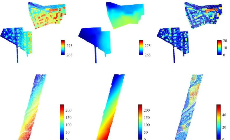
approxi-mation of the scene topography and estimated from the point cloud itself as shown in Figure 2. First, absolute height min-ima are determined on a large grid with a sampling distance of 20m. Afterwards, a linear interpolation is performed among those coarsely gridded minimum values and evalu-ated on a fine grid of0.5m sampling distance. Finally, a normalized height value is assigned to each 3D point by cal-culating the difference of the points’ height value and the topographic height value of the corresponding grid cell.
This yields 62 features per neighborhood parameterized by a fixed radius, 63 features for a neighborhood determined via eigenentropy-based scale selection, and the normalized height feature that is used in addition to each of these neighborhoods.
3.3 Feature Normalization
It is obvious that – by definition – the considered features address different quantities and may therefore be associated with differ-ent units as well as a differdiffer-ent range of values. This, in turn, might have a negative impact on the classification results as the distribution of single classes in the feature space might be sub-optimal. Accordingly, it is desirable to introduce a normalization which allows to transfer the given feature vectors to a new feature space where each feature contributes approximately the same, in-dependent of its unit and its range of values. For this purpose, we conduct a normalization of all features. For the covariance features, the geometric 3D properties and the normalized height feature, we use a linear mapping to the interval[0,1]. To reduce the effect of outliers, the range of the data is determined by the 1st-percentile and the99th-percentile of the training data (Blom-ley et al., 2016a,b). For the shape distributions, the normalization is achieved by dividing each histogram count by the total number of pulls from the local neighborhood (i.e. by255in our case).
3.4 Classification
To classify the derived feature vectors, we employ a Random Forest (RF) classifier (Breiman, 2001) which is a representative of modern discriminative methods (Schindler, 2012) and a good trade-off between classification accuracy and computational ef-fort (Weinmann et al., 2015). The RF classifier relies on ensem-ble learning in terms of strategically combining the hypotheses of a set of weak learners represented by decision trees. The train-ing of such a classifier consists in selecttrain-ing random subsets of the training data and training one decision tree per subset. Thus, the class label for an unseen feature vector can robustly be predicted by considering the majority vote across the individual hypotheses of single decision trees. The internal settings of the RF classifier are determined based on the training data via optimization on a suitable search space.
4. EXPERIMENTAL RESULTS
To evaluate the performance of our framework, we use differ-ent benchmark datasets (Section 4.1), and we consider commonly used evaluation metrics (Section 4.2) to quantitatively assess the quality of the derived classification results (Section 4.3).
4.1 Datasets
To allow for both an objective performance evaluation and an im-pression about how our methodology is able to deal with ALS data of different characteristics, we test our framework on two labeled benchmark datasets which are publicly available and for which no information on the DTM is provided. One dataset is given with theVaihingen Dataset (Section 4.1.1) and the other dataset is given with theGML Dataset A(Section 4.1.2).
4.1.1 Vaihingen Dataset: The Vaihingen Dataset (Cramer, 2010; Rottensteiner et al., 2012) is provided by theGerman So-ciety for Photogrammetry, Remote Sensing and Geoinformation (DGPF) and freely available upon request1. This dataset has been acquired with a Leica ALS50 system over Vaihingen, a small vil-lage in Germany, and corresponds to a scene with small multi-story buildings and many detached buildings surrounded by trees. In the scope of theISPRS Benchmark on 3D Semantic Labeling, a reference labeling has been performed with respect to nine se-mantic classes represented byPowerline,Low Vegetation, Imper-vious Surfaces, Car, Fence/Hedge, Roof, Fac¸ade, Shruband Tree. Thereby, the pointwise reference labels have been deter-mined based on (Niemeyer et al., 2014). For this dataset con-taining about1.166M points in total, a split into a training scene (about754k points) and a test scene (about412k points) is pro-vided as indicated in Table 1. As the reference labels are only provided for the training data and missing for the test data, the results derived with our framework have been submitted to the organizers of the ISPRS Benchmark on 3D Semantic Labeling who performed the evaluation externally.
4.1.2 GML Dataset A: TheGML Dataset A(Shapovalov et al., 2010) is provided by the Graphics & Media Lab, Moscow State University, and publicly available2. This dataset has been acquired with an ALTM 2050 system (Optech Inc.) and contains about2.077M labeled 3D points, whereby the reference labeling
1
http://www2.isprs.org/commissions/comm3/wg4/3d-semantic-labeling.html (visited in April 2017)
2http://graphics.cs.msu.ru/en/science/research/3dpoint/classification
Figure 2. Effects of the scene topography. The point clouds’ height minima on a0.5m grid are shown on the left, the approximation of the scene topography is plotted in the middle, and the normalized minima are shown on the right. The top row depicts the test area of theVaihingen Dataset, while the bottom row shows the test area of theGML Dataset A.
Class Training Data Test Data
Powerline 546 N/A
Low Vegetation 180,850 N/A
Impervious Surfaces 193,723 N/A
Car 4,614 N/A
Fence/Hedge 12,070 N/A
Roof 152,045 N/A
Fac¸ade 27,250 N/A
Shrub 47,605 N/A
Tree 135,173 N/A
Σ 753,876 411,722
Table 1. Number of 3D points per class for theVaihingen Dataset. Note that the reference labels are only provided for the training data and not available for the test data.
Class Training Data Test Data Ground 557,142 439,989
Building 98,244 19,592
Car 1,833 3,235
Tree 381,677 531,852
Low Vegetation 35,093 7,758
Σ 1,074,569 1,002,668
Table 2. Number of 3D points per class for theGML Dataset A. Note that the reference labels are provided for both the training data and the test data.
has been performed with respect to five semantic classes repre-sented byGround,Building,Car,TreeandLow Vegetation. For this dataset, a split into a training scene and a test scene is pro-vided as indicated in Table 2.
4.2 Evaluation Metrics
To evaluate the performance of our framework, we consider com-monly used evaluation metrics that allow quantifying the quality of derived classification results on a per-point basis. On the one hand, we consider global evaluation metrics represented by over-all accuracy OA and the unweighted average of the F1-scores
across all classes (F¯1). As an imbalanced distribution of the
oc-currence of single classes might introduce a bias in the global evaluation metrics, we also consider the classwise evaluation metrics represented by recallR, precisionPandF1-score, where
the latter is a compound metric combining precision and recall with equal weights.
4.3 Results
When training the RF classifier, we take into account that an unbalanced distribution of training examples across all classes might have a detrimental effect on the training process. To avoid this, we randomly sample an identical number of10,000training examples per class for the training phase. Note that this results in a duplication of training examples for those classes for which less training examples are available.
In the testing phase, we focus on the RF-based classification re-lying on geometric features extracted from single neighborhoods and combined neighborhoods. The achieved values for the global evaluation metrics represented by OA andF¯1are provided in
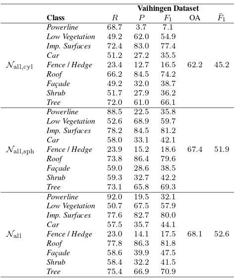
Ta-ble 3 for theVaihingen Datasetand theGML Dataset A. It can be observed that the combination of features extracted from all neighborhoods yields the best classification results. For the com-bined cylindrical neighborhoods (Nall,cyl), the combined spheri-cal neighborhoods (Nall,sph) and the combination of all defined neighborhoods (Nall), the classwise evaluation metrics of recall
R, precisionPandF1-score are provided in Table 4 for the
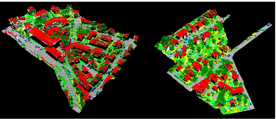
Vai-hingen Datasetand in Table 5 for theGML Dataset A. For the Vaihingen Dataset, it can be observed that the classesImpervious Surfaces,Roof andTreecan be well-detected, whereas particu-larly the classesPowerlineandFence/Hedgeare not appropri-ately identified. For theGML Dataset A, the classesGroundand Treecan be well-detected, whereas particularly the classesCar andLow Vegetationare not appropriately identified. The classi-fication results relying on the use of all defined neighborhoods (Nall) are visualized in Figure 3 for theVaihingen Datasetand in
Figure 3. Classified point cloud for theVaihingen Datasetwith nine classes (Roof: red;Fac¸ade: white;Impervious Surfaces: gray; Car: blue;Tree: dark green;Low Vegetation: bright green;Shrub: yellow;Fence/Hedge: cyan;Powerline: black).
Figure 4. Classified point cloud for theGML Dataset Awith five classes (Ground: gray;Building: red;Car: blue;Tree: dark green; Low Vegetation: bright green).
Vaihingen Dataset GML Dataset A Neighborhood OA F¯1 OA F¯1 Ncyl
,1m
56.5 40.3 81.0 45.4
Ncyl
,2m
57.9 41.3 82.7 46.8
Ncyl
,3m
54.4 37.3 84.3 47.7
Ncyl
,5m
52.9 34.9 86.6 49.3
Nsph
,1m
60.4 42.8 78.4 45.2
Nsph
,2m
62.4 44.5 81.5 48.3
Nsph
,3m
60.3 42.9 84.4 50.5
Nsph
,5m
55.9 37.5 86.7 51.7
Nsph
,kopt
61.7 43.2 83.0 49.1
Nall
,cyl
62.2 45.2 87.7 53.3
Nall
,sph
67.4 51.9 88.3 57.1
Nall 68.1 52.6 90.5 58.5
Table 3. OA andF¯1(in %) achieved for different neighborhood
definitions on theVaihingen Datasetand theGML Dataset A.
5. DISCUSSION
The derived classification results reveal that theGML Dataset A with five semantic classes is not too challenging, as an overall accuracy of about87-91% can be achieved when using the com-bined neighborhoods. This is due to the fact that the dominant
classesGroundandTreecan be accurately classified, whereas the problematic classesCarandLow Vegetationdo not occur that of-ten. In contrast, theVaihingen Datasetwith nine semantic classes is much more challenging which can be verified by an overall ac-curacy of about62-69%. The reason for the lower numbers is that the defined classes are characterized by a higher geometric simi-larity. Particularly the classesLow Vegetation,ShrubandFence/ Hedgeexhibit a similar geometric behavior and misclassifications among these classes therefore occur quite often. However, this is in accordance with other investigations involving theVaihingen Dataset(Blomley et al., 2016a; Steinsiek et al., 2017). Further-more, the classesPowerlineandCarreveal lower detection rates, which is also due to the fact that these classes are not covered representatively in the training data, where they are represented by546and4614examples, respectively.
Vaihingen Dataset
Table 4. Classwise recall (R), precision (P) andF1-score (in %)
as well as OA andF¯1(in %) for theVaihingen Dataset.
spherical neighborhood (Blomley et al., 2016a,b). On the other hand, the results of a pointwise classification are comparable to the ones presented in (Steinsiek et al., 2017) for RF-based classi-fication. While our results are2.9% lower in OA, they are2.6% higher inF¯1. The latter indicates that our framework allows for
a better classification of the different classes, while the approach presented by Steinsiek et al. (2017) allows for a better classifica-tion of the dominant classes as shown in Table 6. To further im-prove the classification results, spatial regularization is required (Landrieu et al., 2017), which has also been taken into account in (Steinsiek et al., 2017; Niemeyer et al., 2014) by using a Condi-tional Random Field (CRF). However, since our framework for pointwise classification allows for a better classification of differ-ent classes, the initial labeling which serves as input to the CRF via the association potentials might be improved which, in turn, is likely to allow the CRF to further increase the quality of the classification results.
6. CONCLUSIONS
In this paper, we have presented a novel framework for semanti-cally labeling 3D point clouds acquired via airborne laser scan-ning. The framework uses a combination of multiple cylindrical and multiple spherical neighborhoods to extract geometric tures in the form of both metrical features and distribution fea-tures at different scales. Furthermore, we used neighborhoods in the form of spatial bins to approximate the topography of the considered scene and thus obtain normalized heights. All fea-tures have been normalized and provided as input to a Random Forest classifier. The results achieved for two commonly used benchmark datasets clearly revealed the potential of the proposed methodology for pointwise classification. The improvement with respect to related investigations on pointwise semantic labeling also represents an important prerequisite for a subsequent
spa-GML Dataset A
Table 5. Classwise recall (R), precision (P) andF1-score (in %)
as well as OA andF¯1(in %) for theGML Dataset A.
for theVaihingen Dataset(1result presented by Steinsiek et al.
(2017);2result achieved with the proposed framework).
tial regularization. In future work, it would be desirable to inte-grate spatial regularization techniques such as the ones presented in (Landrieu et al., 2017; Niemeyer et al., 2014; Steinsiek et al., 2017). This would impose spatial regularity on the derived classi-fication results and thus improve them significantly. Furthermore, the step from a classification on a per-point basis to the detection of individual objects in the scene would be interesting as this fa-cilitates an object-based scene analysis.
ACKNOWLEDGEMENTS
The Vaihingen Dataset was kindly provided by the German Society for Photogrammetry, Remote Sensing and Geoin-formation (DGPF) (Cramer, 2010): http://www.ifp.uni-stuttgart.de/dgpf/DKEP-Allg.html.
References
Blomley, R., Jutzi, B. and Weinmann, M., 2016a. 3D semantic labeling of ALS point clouds by exploiting multi-scale, multi-type neighborhoods for feature extraction. In:Proceedings of the International Conference on Geographic Object-Based Image Analysis, Enschede, The Nether-lands, pp. 1–8.
Blomley, R., Jutzi, B. and Weinmann, M., 2016b. Classification of air-borne laser scanning data using geometric multi-scale features and dif-ferent neighbourhood types. In:ISPRS Annals of the Photogrammetry, Remote Sensing and Spatial Information Sciences, Prague, Czech Re-public, Vol. III-3, pp. 169–176.
Brodu, N. and Lague, D., 2012. 3D terrestrial lidar data classification of complex natural scenes using a multi-scale dimensionality criterion: applications in geomorphology. ISPRS Journal of Photogrammetry and Remote Sensing68, pp. 121–134.
Chehata, N., Guo, L. and Mallet, C., 2009. Airborne lidar feature se-lection for urban classification using random forests. In: The Inter-national Archives of the Photogrammetry, Remote Sensing and Spatial Information Sciences, Paris, France, Vol. XXXVIII-3/W8, pp. 207– 212.
Cramer, M., 2010. The DGPF-test on digital airborne camera evaluation – Overview and test design.PFG Photogrammetrie – Fernerkundung – Geoinformation2 / 2010, pp. 73–82.
Demantk´e, J., Mallet, C., David, N. and Vallet, B., 2011. Dimensionality based scale selection in 3D lidar point clouds. In:The International Archives of the Photogrammetry, Remote Sensing and Spatial Infor-mation Sciences, Calgary, Canada, Vol. XXXVIII-5/W12, pp. 97–102.
Filin, S. and Pfeifer, N., 2005. Neighborhood systems for airborne laser data. Photogrammetric Engineering & Remote Sensing71(6), pp. 743–755.
Gevaert, C. M., Persello, C. and Vosselman, G., 2016. Optimizing multi-ple kernel learning for the classification of UAV data.Remote Sensing
8(12), pp. 1–22.
Grilli, E., Menna, F. and Remondino, F., 2017. A review of point clouds segmentation and classification algorithms. In: The International Archives of the Photogrammetry, Remote Sensing and Spatial Infor-mation Sciences, Nafplio, Greece, Vol. XLII-2/W3.
Guo, B., Huang, X., Zhang, F. and Sohn, G., 2015. Classification of airborne laser scanning data using JointBoost.ISPRS Journal of Pho-togrammetry and Remote Sensing100, pp. 71–83.
Guo, L., Chehata, N., Mallet, C. and Boukir, S., 2011. Relevance of air-borne lidar and multispectral image data for urban scene classification using random forests.ISPRS Journal of Photogrammetry and Remote Sensing66(1), pp. 56–66.
Hackel, T., Wegner, J. D. and Schindler, K., 2016. Fast semantic seg-mentation of 3D point clouds with strongly varying density. In:ISPRS Annals of the Photogrammetry, Remote Sensing and Spatial Informa-tion Sciences, Prague, Czech Republic, Vol. III-3, pp. 177–184.
Hu, H., Munoz, D., Bagnell, J. A. and Hebert, M., 2013. Efficient 3-D scene analysis from streaming data. In:Proceedings of the IEEE In-ternational Conference on Robotics and Automation, Karlsruhe, Ger-many, pp. 2297–2304.
Jutzi, B. and Gross, H., 2009. Nearest neighbour classification on laser point clouds to gain object structures from buildings. In: The Inter-national Archives of the Photogrammetry, Remote Sensing and Spatial Information Sciences, Hannover, Germany, Vol. XXXVIII-1-4-7/W5.
Khoshelham, K. and Oude Elberink, S. J., 2012. Role of dimensionality reduction in segment-based classification of damaged building roofs in airborne laser scanning data. In:Proceedings of the International Con-ference on Geographic Object Based Image Analysis, Rio de Janeiro, Brazil, pp. 372–377.
Kraus, K. and Pfeifer, N., 1998. Determination of terrain models in wooded areas with airborne laser scanner data.ISPRS Journal of Pho-togrammetry and Remote Sensing53(4), pp. 193–203.
Landrieu, L., Mallet, C. and Weinmann, M., 2017. Comparison of belief propagation and graph-cut approaches for contextual classification of 3D lidar point cloud data. In: Proceedings of the IEEE Geoscience and Remote Sensing Symposium, Fort Worth, USA, pp. 1–4.
Lee, I. and Schenk, T., 2002. Perceptual organization of 3D surface points. In: The International Archives of the Photogrammetry, Re-mote Sensing and Spatial Information Sciences, Graz, Austria, Vol. XXXIV-3A, pp. 193–198.
Linsen, L. and Prautzsch, H., 2001. Local versus global triangulations. In:Proceedings of Eurographics, Manchester, UK, pp. 257–263.
Lodha, S. K., Fitzpatrick, D. M. and Helmbold, D. P., 2007. Aerial lidar data classification using AdaBoost. In: Proceedings of the Interna-tional Conference on 3-D Digital Imaging and Modeling, Montreal, Canada, pp. 435–442.
Lodha, S. K., Kreps, E. J., Helmbold, D. P. and Fitzpatrick, D., 2006. Aerial lidar data classification using support vector machines (SVM). In:Proceedings of the International Symposium on 3D Data Process-ing, Visualization, and Transmission, Chapel Hill, USA, pp. 567–574.
Mallet, C., Bretar, F., Roux, M., Soergel, U. and Heipke, C., 2011. Rel-evance assessment of full-waveform lidar data for urban area classifi-cation.ISPRS Journal of Photogrammetry and Remote Sensing66(6), pp. S71–S84.
Mongus, D. and ˇZalik, B., 2012. Parameter-free ground filtering of Li-DAR data for automatic DTM generation. ISPRS Journal of Pho-togrammetry and Remote Sensing67, pp. 1–12.
Niemeyer, J., Rottensteiner, F. and Soergel, U., 2014. Contextual classifi-cation of lidar data and building object detection in urban areas.ISPRS Journal of Photogrammetry and Remote Sensing87, pp. 152–165.
Osada, R., Funkhouser, T., Chazelle, B. and Dobkin, D., 2002. Shape distributions.ACM Transactions on Graphics21(4), pp. 807–832.
Pauly, M., Keiser, R. and Gross, M., 2003. Multi-scale feature extraction on point-sampled surfaces.Computer Graphics Forum22(3), pp. 81– 89.
Rottensteiner, F., Sohn, G., Jung, J., Gerke, M., Baillard, C., Benitez, S. and Breitkopf, U., 2012. The ISPRS benchmark on urban object classification and 3D building reconstruction. In:ISPRS Annals of the Photogrammetry, Remote Sensing and Spatial Information Sciences, Melbourne, Australia, Vol. I-3, pp. 293–298.
Rusu, R. B., Blodow, N. and Beetz, M., 2009. Fast point feature his-tograms (FPFH) for 3D registration. In: Proceedings of the IEEE International Conference on Robotics and Automation, Kobe, Japan, pp. 3212–3217.
Schindler, K., 2012. An overview and comparison of smooth labeling methods for land-cover classification. IEEE Transactions on Geo-science and Remote Sensing50(11), pp. 4534–4545.
Schmidt, A., Niemeyer, J., Rottensteiner, F. and Soergel, U., 2014. Con-textual classification of full waveform lidar data in the Wadden Sea.
IEEE Geoscience and Remote Sensing Letters11(9), pp. 1614–1618.
Shapovalov, R., Velizhev, A. and Barinova, O., 2010. Non-associative Markov networks for 3D point cloud classification. In: The Inter-national Archives of the Photogrammetry, Remote Sensing and Spa-tial Information Sciences, Saint-Mand´e, France, Vol. XXXVIII-3A, pp. 103–108.
Sithole, G. and Vosselman, G., 2004. Experimental comparison of filter algorithms for bare-Earth extraction from airborne laser scanning point clouds.ISPRS Journal of Photogrammetry and Remote Sensing 59(1-2), pp. 85–101.
Steinsiek, M., Polewski, P., Yao, W. and Krzystek, P., 2017. Semantische Analyse von ALS- und MLS-Daten in urbanen Gebieten mittels Con-ditional Random Fields. In: Tagungsband der 37. Wissenschaftlich-Technischen Jahrestagung der DGPF, W¨urzburg, Germany, Vol. 26, pp. 521–531.
Tombari, F., Salti, S. and Di Stefano, L., 2010. Unique signatures of histograms for local surface description. In: Proceedings of the Eu-ropean Conference on Computer Vision, Heraklion, Greece, Vol. III, pp. 356–369.
Vosselman, G., Gorte, B. G. H., Sithole, G. and Rabbani, T., 2004. Recog-nising structure in laser scanner point clouds. In: The International Archives of the Photogrammetry, Remote Sensing and Spatial Infor-mation Sciences, Freiburg, Germany, Vol. XXXVI-8/W2, pp. 33–38.
Weinmann, M., 2016.Reconstruction and analysis of 3D scenes – From irregularly distributed 3D points to object classes. Springer, Cham, Switzerland.
Weinmann, M., Jutzi, B., Hinz, S. and Mallet, C., 2015. Semantic point cloud interpretation based on optimal neighborhoods, relevant features and efficient classifiers. ISPRS Journal of Photogrammetry and Re-mote Sensing105, pp. 286–304.
West, K. F., Webb, B. N., Lersch, J. R., Pothier, S., Triscari, J. M. and Iverson, A. E., 2004. Context-driven automated target detection in 3-D data.Proceedings of SPIE5426, pp. 133–143.
Xu, S., Vosselman, G. and Oude Elberink, S., 2014. Multiple-entity based classification of airborne laser scanning data in urban areas. ISPRS Journal of Photogrammetry and Remote Sensing88, pp. 1–15.