Accounting Fundamentals and the Variation of Stock Price: Factoring in the Investment Scalability | Sumiyana | Gadjah Mada International Journal of Business 5508 9387 1 PB

Gadjah Mada International Journal of Business May­August 2010, Vol. 12, No. 2, pp. 189–229

Sumiyana

Zaki Baridwan

Slamet Sugiri

Jogiyanto Hartono M.

All  of  authors  are  from  Faculty  of  Economics  and  Business,  Universitas  Gadjah  Mada

ACCOUNTING FUNDAMENTALS AND

THE VARIATION OF STOCK PRICE

Factoring in the Investment Scalability

*

This study develops a new return model with respect to accounting fundamentals. The new return model is based on Chen and Zhang (2007). This study takes into account the investment scalability information. Specifically, this study splits the scale of firm’s operations into short-run and long-run investment scalabilities. We document that five accounting fun-damentals explain the variation of annual stock return. The factors, comprised book value, earnings yield, short-run and long-run investment scalabilities, and growth opportunities, co-associate positively with stock price. The remaining factor, which is the pure interest rate, is negatively related to annual stock return. This study finds that inducing short-run and long-run investment scalabilities into the model could improve the

Introduction

Chen  and  Zhang  (2007)  present the latest return model that relates the fundamental firm value to the variation in stock price. They also provide theo­ retical and empirical evidence that stock return is a function of accounting vari­ ables,  namely  earnings  yield,  equity capital,  the  change  in  profitability, growth opportunities, and discount rate. Chen and Zhang (2007) argue that firm value embraces information on poten­ tial future assets and growth opportuni­ ties.  This  argument  is  supported  by Miller and Modigliani (1961). In a simple explanation, both studies infer that stock price is a function of future assets or capital scalability.1 _{Earnings could be}

determined by the adaptation concept when the firm’s invested resources are modifiable to generate future earnings (Wright 1967).

The  association  between  stock return and fundamental firm value has

been  examined  by  Burgstahler  and Dichev (1997) and Collins et al. (1999). They suggest that earnings yield has a concave­nonlinear association, thereby not purely linear. Other studies show otherwise,  an  inverse  relationship  of earnings and book value of equity to stock price or return (Jan and Ou 1995, and Collins et al. 1999). The inconsis­ tent  relationship  between  stock  price and accounting fundamentals has been overviewed by Lev (1989), Lo and Lys (2000), and Kothari (2001). Those re­ searchers argue that this inconsistency is due to: (1) a weak relationship be­ tween  earnings  and  stock  price  vari­ ability, marked by R2 _{less than 10}

per-cent (Chen and Zhang 2007), and (2) a linear correlation between accounting information  and  future  related  cash flows, with equity value as a function of scalability  and  profitability  (Ohlson 1995; Feltham and Ohlson 1995, 1996; Zhang  2003;  and  Chen  and  Zhang 2007).

Keywords: accounting fundamentals; book value; earnings yield; growth opportuni­ ties;  short­run  and  long­run  investment  scalabilities;  trading  strategy; value relevance

JEL Classification: M41 (accounting); G12 (assets pricing; interest rate); G14 (information and market efficiency); G15 (international financial markets)

degree of association. In other words, they have value rel-evance. Finally, this study suggests that basic trading strategies will improve if investors revert to the accounting fundamentals.

1 _{Scalability is actually a firm’s scale of operations. This study shortens it into scalability. It refers}

This study  is mainly  focused on designing a new return model and ex­ amining  the  model.  Previous  studies clearly show a positive association be­ tween accounting data and return based on  four  related  cash  flows,  namely earnings yield, equity capital, profitabil­ ity,  and  growth  opportunities,  and  a negative relationship with the costs of debt and equity capital (Zhang 2003, and  Chen  and  Zhang  2007).  Since previous models have yet to compre­ hensively  explain  the  role  of  equity capital, this recently designed model is aimed at enhancing the identification of initial factors causing the equity capital scalability to rise, whether it is short­ run or long­run investment scalability according  to  financial  management concepts (Smith 1973).

Hatsopoulus (1986) supports the investment scalability argument, sug­ gesting that the strength of firm pro­ ductivity  is  associated  with  earnings and stock price. Drucker (1986) also concludes  that  production  scalability affects not only the earnings power but also  the  firm’s  market  value.  Other empirical studies  have confirmed  the followings: (1) the positive association between assets productivity and equity value (Kaplan 1983), (2) the efficient productivity shown by low­cost assets usage  to  increase  the  firm’s  equity (Dogramaci 1981; Kendrick 1984), (3) the  cheap­resource  inputs  to  ensure future  growth  of  the  firm  (Kendrick 1984),  (4)  the  enhancement  of  firm productivity to improve the firm’s eq­ uity value and stockholder wealth (Bao and Bao 1989), and (5) the non­earn­

ings numbers as an additional predic­ tive value, which is called the valuation link (Ou 1990).

This complementary analysis re­ lies on the following reasons. First, the limitation  of  Ohlson’s  (1995)  model (Feltham and Ohlson 1995, 1996). This weakness lies in its assumptions that: (i) future earnings could be determined using  consecutive  previous  earnings and  (ii)  earnings  could  be  pre­deter­ mined  stochastically. Second,  earn­ ings  is  a  noise  when  measuring  eco­ nomic earnings and equity value (Kolev et al. 2008; Collins et al. 1997; Givoly and  Hayn  2000;  and  Bradshaw  and Sloan 2002). Third, high value is rel­ evant  when  eliminating  earnings (Bradshaw  and  Sloan  2002;  and Bhattacharya et al. 2003). Therefore, this  study  provides  complementary measurement  of  earnings.  Addition­ ally, this study is focused on the adap­ tation  theory  in  which  assets  on  the statement  of  financial  position  are  a determinant  of  equity  value (Burgstahler and Dichev 1977).

2003, and Chen and Zhang 2007), but it also investigates further by factoring in the short­run and long­run investment scalabilities. This study examines the new  theoretical  return  model  using empirical  data.  Furthermore,  robust­ ness checks are conducted to confirm the consistency between the new model and its predecessors, including the as­ sociation between each construct and stock return.

This study benefits both investors and  managers.  From  the  investor’s point of view, this study provides more comprehensive, realistic, and accurate parameters for predicting potential fu­ ture  cash flows  since  the new  model extracts more information than do cur­ rently  available  models.  From  the manager’s  point  of  view,  this  study gives  incentives  to  managers  to  dis­ close  more  information  publicly  as mandated by SFAC No. 5, paragraph 24 (FASB 1984). Finally, the new re­ turn model can lead investors and man­ agement  to  assess  comprehensively the information conveyed in financial statements.

This study contributes to account­ ing literature by providing more com­ plete and realistic return model. This study has advantages compared with the models of Easton and Harris (1991), Liu and Thomas (2000), Zhang (2003), Copeland et al. (2004), Chen and Zhang (2007),  and  Weiss et  al.  (2008),  ex­ plained as follows. First, this model is more comprehensive due to its broader coverage, specifically the inclusion of assets  scalability  to  generate  future cash flows.

Second, by including scalability,

this model is expected to be closer to the  economic  reality  as  firms  should reasonably  choose  future  investment projects that will contribute positive net cash  inflow.  Cash  inflow  magnifies earnings and its variability. The second advantage  is  labeled  as  the  earnings capitalization model by Ohlson (1995), who explains that earnings and its vari­ ability are affected by current projects.

Third, the new return model cre­

ates a more comprehensive and accu­ rate predictor of future cash flows to estimate  potential  future  earnings  by extracting  multiple  relevant  informa­ tion (Liu et al. 2001). Multiple informa­ tion could improve model accuracy as long  as  it  is  aligned  with  increasing value relevance. Eventually, this study offers  considerable  contribution  by improving the degree of association of return model as it is more comprehen­ sive, realistic, and accurate. This con­ tribution is reflected by higher R2 _and

adj-R2 _{than the previous models.}

assets  as  the  stimulus  for  increasing the firm’s equity value. This refers to the adaptation theory (Wright 1967).

Fourthly, the efficiency form of stock

market is comparable. Stock price vari­ ability on all stock markets acts in the same  market­wide  regime  behavior, and depends solemnly on earnings and book value (Ho  and Sequeira 2007).

Fifthly,  cost  of  equity  capital  repre­

sents  the  opportunity  cost  for  each firm.  It  suggests  that  every  fund  is managed in order to maximize assets usability and that management always behaves rationally.

Literature Review, Models

and Hypotheses Development

Earnings Yield and Stock Value

Ohlson  (1995)  reveals  that  firm equity  comes  from  book  value  and future residual value. Firm value can be  calculated  from  current,  potential discount  rate  which  is  unrelated  to current  accounting  net  capital  eco­ nomic  assets.  If  a  firm  creates  new wealth value from invested assets, the new wealth value is concluded in the firm’s net equity capital. Hence, this net value is reflected in the firm’s stock price.

Ohlson’s  (1995)  model  suggests linear  information  dynamics  of  book value  and  expected  residual  value  in association with stock price. This model was  then  followed  by  a  myriad  of further studies. Lo and Lys (2000), and Myers (1999) implemented the linear information  dynamics  model  for  the

first  time,  which  is  afterwards  re­ nowned  as  the  clean  surplus  theory. This theory argues that year­end stock price is the result of beginning­of­the­ year stock price added by current earn­ ings  and  subtracted  by  current  divi­ dends  paid.  Meanwhile,  Lundholm (1995)  finds  that  the  firm’s  market value  is  the  sum  of  invested  equity capital and its future residual earnings discounted by the cost of invested capi­ tal.

Other  research  has  consistently utilized Ohlson’s (1995) model without criticizing the stock value and earnings within the model. Feltham and Ohlson (1995; 1996) emphasize that the asso­ ciation between stock value and earn­ ings is asymptotic. This relation may be affected by other information and ac­ counting conservatism in depreciation. Burgstahler  and  Dichev  (1997)  used the  same  model,  and  introduced  the book values of assets and debt to better explain  firm  value.  Liu  and  Thomas (2000)  and  Liu  et  al.  (2001)  added multiple factors, both earnings disag­ gregating and other measures related to  book  value  and  earnings,  into  the clean surplus model.

ings quality improves return associa­ tion. Collins et al. (1999) declare simi­ lar conclusion, and enhance the asso­ ciation by eliminating firms with nega­ tive earnings.

Prior to  Ohlson’s (1995)  model, research  in  the  past  had  associated book value and earnings with the firm’s market  value.  Rao  and  Litzenberger (1971) and Litzenberger and Rao (1972) provide evidence that the firm’s mar­ ket value is a function of book value and earnings although the relation might be adjusted by the functions of debt and productivity  growth.  Bao  and  Bao (1989) specifically indicate that equity is  not  only affected  by  earnings,  but also  by  expected  earnings,  standard deviation  of  earnings,  and  earnings growth.

Investment Scalability

The first limitation  of  Ohlson’s

(1995) model lies in its assumptions. Continued  by  Feltham  and  Ohlson (1995; 1996), it still assumes that future earnings is determined by consecutive previous earnings. However, investors may have different insights by observ­ ing  future  potential  earnings. Burgstahler and Dichev (1977) clearly reveal that equity value is not affected by previous earnings only, but could be determined by the adaptation theory,2

which  is  the  firm’s  invested  capital when its resources are modifiable for other utilizations. Furthermore, the other

utilizations may generate future poten­ tial earnings. This concept is based on Wright  (1967),  who  argues  that  the adaptation  value  is  derived  from  the role  of  financial  information  on  the balance sheet,  and the  role primarily comes  from  assets.

The second limitation of Ohlson’s

model (Ohlson 1995; and Feltham and Ohlson 1995, 1996) lies in its earnings assumption. Earnings is assumed to be pre­determined  stochastically.  This concept  is  based  on  Sterling  (1968), assuming that firms are in stationary condition. The concept basically postu­ lates that a firm continues to operate based on its past strength and perfor­ mance. In fact, the firm’s strength and performance may change due to tech­ nology, merger and acquisition, take­ over, liquidation, bankruptcy, restruc­ turing, management turnover, and new invested capital.

Ohlson (1995; 2001) himself ad­ mitted  to  the  limitations,  citing  that there was other information noted as a mysterious  variable.  This  variable makes the stock markets fail to reflect book value, or lessens the information content.  Further  research  has  been attempting  to  replace  the  mysterious variable (e.g., Beaver 1999; Hand 2001), although both of those studies are merely an interpretative commentary or evalu­ ative review of the Ohlson’s model.

Later  research  has  left  Ohlson’s concept and tried to complement it with

2  _{Apart  of  the  adaptation  theory,  another  approach  to  determining  firm  equity  value  is  the}

other  empirical  models.  Francis  and Schipper  (1999)  have  abandoned Ohlson’s linear information dynamics by  adding  assets  and  debt  into  the return  model.  This  addition  has  em­ barked on measuring assets scalability in either long or short run. Abarbanell and Bushee (1997) modified the return model by adding fundamental signals, and their changes consist of invento­ ries,  accounts  receivable,  capital  ex­ penditures,  gross  profit,  and  taxes. These  fundamental  signals  represent investment scalability from assets on the statement of financial position.

Bradshaw et al. (2006) modified Ohlson’s return model by inducing the magnitude of financing obtained from debt.  This  change  in  debt  is  compa­ rable to the change in assets utilized to generate  earnings.  Cohen  and  Lys (2006)  improved  the  model  by Bradshaw et al. (2006) by inducing not only  the  change  in  debt  but  also  the change  in  short­run  investment scalability, which is the change in in­ ventories.  Heretofore,  long­run  and short­run investment scalabilities have been  put  into  consideration.  Mean­ while, Weiss et al. (2008) emphasize the  short­run  investment  scalability, which  are  the  changes  in  inventories and accounts receivable to improve the degree of association.

Before  Ohlson’s  (1995)  model, short­run  and  long­run  investment scalabilities had been associated with equity value. Bao and Bao (1989) con­ struct production capacities measured by  the  economic  value  added,  which are  the  changes  in  inventories  and

direct  labor  costs  to  measure  short­ term productivity and fixed assets de­ preciation  to  measure  long­term  ca­ pacity.

Accounting  earnings  as  a  noise when  measuring  economic  earnings and equity was introduced by Kolev, Marquadt and McVay (2008), Collins et al. (1997), Givoly and Hayn (2000), and Bradshaw and Sloan (2002). An investor  adjusts  his  or  her  focus  to earnings  not  based  on  the  generally accepted accounting principles, but in­ stead  on  the  measurement  of  core potential earnings. Compelling results from  the  studies  of  Bradshaw  and Sloan (2002) and Bhattacharya et al. (2003) indicate that earnings is elimi­ nated to improve the value relevance of their return models.

Changes in Growth

Opportunities

Ohlson’s (1995) model maintains the clean surplus theory which relates accounting information to the following premises:  (1)  stock  market  value  is based on discounted future dividends in which investors have a neutral position against risk, (2) accounting information is sufficient to calculate clean surplus, and (3) future earnings is stochastic, pre­determined by consecutive previ­ ous earnings. However, investors may respond  differently  to  minimum  or maximum profitability. Hence, growth factors, as have been included by other research, may  affect earnings.

Rao  and  Litzenberger  (1971), Litzenberger and Rao (1972), and Bao and Bao (1972) conclude that growth and its change increase firm competi­ tiveness. Consequently, the higher the efficiency, the higher the productivity and accordingly the higher the stock­ holder  and  country  wealth.  Rao  and Litzenberger (1971) and Litzenberger and  Rao  (1972)  specifically  disclose that growth opportunities are directly associated with long­run prospect within one industry. Those studies are based on Miller and Modigliani (1961), con­ cluding that growing firm is a firm that has a positive rate of return for each invested  capital.  It  also  means  that every  invested  resource  has  a  lower cost  of  capital  than  that  within  the industry.

Liu  et  al.  (2001),  Aboody  et  al. (2002),  and  Frankel  and  Lee  (1998) show a perspective that a firm’s intrin­

sic value is determined by growth and future potential growth. Current growth drives the increase in potential future earnings,  whereas  future  potential growth  reduces  the  model’s  residual error to improve the degree of model association.  Lev  and  Thiagarajan (1993), Abarbanell and Bushee (1997), and Weiss et al. (2008) suggest that the growth in inventories, gross profit, sales, accounts receivable, etc. improves fu­ ture earnings growth. Moreover, their research concludes that market value adapts  to  all  the  growth  factors. Danielson and Dowdell (2001) exam­ ined growing firms, and find that they have better financial performance than do other firms. Their study also shows that the P/B ratio of growing firms is greater than that of other companies. Chen and Zhang (2007) find evi­ dence that  firm value  completely de­ pends  on  growth  opportunities.  The growth  opportunities  per  se  are  the function of assets operation scale, and affect  the  potential  to  grow  continu­ ously. The inclusion of growth opportu­ nities is based on the perspective that earnings and book value are not suffi­ cient to explain stock price movement. Therefore, the analysis on current and future earnings could be enhanced when external environment, industry, and in­ terest rate are taken into account.

Changes in Discount Rate

and  Wahlen  (2000).  Their  modifica­ tions lie in the fact that interest rate can change  the  firm’s  future  earnings power.  Related  to  investor’s  percep­ tion,  interest  rate  movement  may change the investor’s belief in the firm’s earnings power since future earnings can be referred to as a set of discount rates giving better certainty of future earnings.

Rao and Litzenberger (1971), and Litzenberger  and  Rao  (1972)  imply that equity value depends on the dis­ count rate of future potential earnings. In  turn,  this  discount  rate  hinges  on pure interest rate, and then affects the efficiency of the firm’s scale of opera­ tions  and finally  earnings.  Danielson and  Dowdell  (2001),  and  Lie  et  al. (2001) find that firm equity is highly affected by expected discount rate to grow assets  and book  value. Interest rate has a multiplier effect. If the inter­ est rate relative to current assets and capital is higher than the pure interest rate, the firm can generate more earn­ ings.  An  alternative  interpretation  is that  the  increase  in  debt  or  new  in­ vested capital could relatively decrease the cost of capital.

Burgstahler  and  Dichev  (1997) suggest  that  a  firm’s  equity  value  is increased  by  the  adaptation  theory. This value may increase by attaining cheaper  alternative  sources,  such  as exploring  alternative  resources  with lower interest rate to improve the firm’s productivity.  Aboody  et  al.  (2002), Frankel and Lee (1998), Zhang (2003) and Chen and Zhang (2007) argue that earnings growth is determined by inter­

est  rate.  It  serves  as  an  adjustment factor to the firm’s scale of operations. In other words, external environment factors  may  affect  earnings  growth, such  as  the  external  interest  rate  se­ lected  by  management  to  make  the operations efficient.

A Model of Equity Value

A  model  of  equity  value  relates accounting information with the pros­ pect  of  future  cash  flows.  This  ap­ proach  was  employed  by  Ohlson (1995), and Feltham and Ohlson (1995; 1996). The model is based on the firm’s scale  of  operations  (scalability)  and profitability. Scalability and profitabil­ ity are a function of current condition and future potential cash flows. Thus, earnings plays a major role due to its ability to show the firm’s tendency to expand operations or to abandon op­ erations. Equity value model is a pro­ cess of measuring equity investment to expand  or  to  cease  operations (Burgstahler and Dichev 1997). Zhang (2003) developed the equity value model that simplified the probability of firm’s going  concern  or  firm’s  abandoning operations.

Zhang (2003) and Chen and Zhang (2007) symbolize the equity value fi­ nanced on date t (end period t) with V_t. Next, X_t  represents  earnings during period t. B_t is the book value of firm equity. E_t(X_t+1) is expected future earn­ ings, k is earnings capitalization factor,

while, g_t is earnings growth opportuni­ ties. Chen and Zhang (2007) formulate equity value as follows.

Model (1) formulates that equity value (V_t) is associated with expected future  earnings  from  invested  assets

(E_t(X_t+1), earnings capitalization factor

(k),  the  probability  of  abandonment option (P(q_t)), and the probability of continuation option (C(q_t)). This model indicates that equity value is equal to the continuation of current operations

(q_t) added by firm growth opportuni­ ties, either positive or negative (g_t).

Based on the model by Chen and Zhang (2007), this study expands their model  by  complementing  and  trans­ forming  it into  a  detailed form.  This transformation  is  supported  by  Ou (1990) who implies that non­earnings accounting value can be used as cur­ rent  and  future  earnings  predictors. Non­earnings information may give an additional predictive value reflected in stock price. Therefore, this study adds the non­earnings values as predictors. The  transformation  is  based  on the  rationale  that q_t  X_t/B_t-1 may  be specified by sr_t and lr_t. Short­run in­ vestment  scalability  is sr_t = (Asr_t

-Lsr_t)/(Asr_t-1-Lsr_t-1), where A is assets

and L is liabilities; and long­run invest­ ment scalability is lr_t = (Alr_t - Llr_t)/ (Alr_t-1-Llr_t-1).  The  transformation  re­ sults in a complete formula expressed in Model (2) as follows.

By transforming q_t into sr_t and lr_t, this  study  develops  a  logical  frame­ work as follows. Parameter q_t as earn­ ings is capital inflow to the firm from its operating activities. Thus, Model (1) is based on the capital cash flows. It is formulated in this study that earnings is measured by assets, symbolized as sr_t

and lr_t. In order to synchronize with the flow  form,  this  study  transforms  the stock form into the flow form by mea­ suring the changes, namely by (Asr_t -Lsr_t) and (Alr_t-Llr_t), and then normal­ izes them on the basis of prior period

(Asr_t-1-Lsr_t-1)  and (Alr_t-1-Llr_t-1).  Sec­ ondly, Zhang (2003) posits that earn­ ings increases due to the firm’s expan­ sion.  This  study  formulates  that  the increase in earnings is not only caused by the firm’s expansion, but also by the scalability of their productive assets. Assets refer to all resources managed to  generate  earnings.  Therefore,  the net  difference  between  assets  and  li­ abilities could be used to measure the firm’s  earnings  power.  Additionally, the transformation of q_t into sr_t and lr_t

is  based  on  Rao  and  Litzenberger (1971), suggesting that the book values of assets and liabilities could increase or decrease the potential future earn­ ings (Smith 1973).

The next step is Model (2) simpli­ fication. Earnings growth usually fol­ lows  the  random walk,  meaning  that

V_t= kE_t(X_t+1) + B_t(P(sr_t) + P(lr_t)) + B_t.g_t(C(sr_t) + C(lr_t))...(2) V_t= kE_t(X_t+1) + B_t.P(q_t) +

earnings growth depends on previous year’s observed earnings. With q_t+1= q_t + e_t+1, with e_t+1 being the mean­error close  to  zero,  then  E_t(X_t+1)= E_t(B_tq_t+1)= B_tq_t,  and  with k = 1/r_t. Assets growth used to generate earn­ ings follows the same pattern as does earnings growth. Transformation of q_t

into sr_t and lr_t results in the following equation.

Substituting  Equation  (3)  into Model (2) results in Equation (4) be­ low.

According to Equation (4), an ad­ dition of one unit of assets or one unit of invested capital into the firm’s equity (v) could increase with a certain mag­ nitude current equity value. Its formu­ lation in Equation (5) is as follows.

A Model of Stock Return

To  develop  a  return  model,  this study considers the equity value model, which assumes that the change in eq­ uity  value  starts  from  date t-1  to t, notated as V_t. To construe Equation (6), the change in firm value is equal to the change in book value of equity as a function of four cash­flow­related fac­ tors (B_tv(sr_t-1, lr_t-1, g_t-1, r_t-1)) and the book value multiplied by the changes in all  four  factors  (sr_t, lr_t, g_t,  and

r_t). Subsequently, return formulation is shown by the following Equation 6.

...(6)

To  show  the  change  in  each  re­ lated factor, the differential equation is

developed  as  follows. 

(

)

1 1





t

sr

d

dv

v

_,

)

(

1

2





t

lr

d

dv

v

_{,  and} 

1 3





t

dr

dv

v

_{,  with}



(

1

)

(

1

)



1  







t t

t

lr

sr

C

dg

dv

.

If the firm pays dividend D_t during period t, the net contribution for current return (R_t) is as follows.

...(7) E_t(X_t+1)= E_t(B_tq_t+1)=  B_tq_t=

B_t((sr_t) +  (lr_t))...(3)

V_t= B_t       + P(sr_t) +

P(lr_t) + g_t(C(sr_t) + C(lr_t)) ...(4)

(sr_t) + (lr_t) r_t

(

(

V_t= B_tv      + P(sr_t) +

P(lr_t) + g_t(C(sr_t) + C(lr_t)) ...(5)

(sr_t) + (lr_t) r_t

(

(

Substituting  Equation  (7)  into Equation (6), an equation to calculate stock return during current period (R_t) is as follows.

Because of       ,

substituting  it  into  Equation  (9)  will obtain Equation (9) as follows.

Assuming that book value growth is equal to earnings during current pe­ riod subtracted by dividend during cur­

rent period, or referred to as the clean surplus relation, then B_t = X_t – D_t. This equation is reversed into D_t = X_t – B_t. If this equation is substituted into Equation (10), it results in the following equation.

Equation  (10)  shows  that  stock return  is  a  function  of  the  following factors: (1) earnings yield (X_t/V_t-1), (2) the change in earnings from short­run invested assets (sr_t), (3) the change in earnings from long­run invested as­ sets  (lr_t),  (4)  the  change  in  book equity value (B_t/B_t-1), (5) the change in growth opportunities (g_t), and (5) the change in discount rate (r_t).

Hypotheses Development

Earnings Yield

Earnings yield (X_t) shows an addi­ tional value generated since the begin­ ning  of  invested  capital  (henceforth,

B_t V_t­1

R_t = v       + v₁      Bt­1 sr_t  

V_t­1 B_t­1

V_t­1

v₂      lr_t     + (C(Sr_t) +

C(lr_t))      B_Vt­1 g_t     +

t­1

v₃      B_Vt­1r_t    +

t­1

D_t V_t­1

...(8)

X_t V_t­1

R_t = v       + v₁      sr_t  

...(10) B_t­1

V_t­1

v₂         lr_t     +  

(

1­       

)      

+ B_t­1

V_t­1

B_t V_t­1

B_t­1 B_t­1

(C(sr_t)) + C(lr_t))        Bt­1g_t     + V_t­1

v₃      Bt­1r_t V_t­1

B_t V_t­1

R_t =       + v₁      Bt­1 sr_t  

V_t­1

(C(Sr_t) + C(lr_t))      Bt­1 g_t    +   V_t­1

v₃      Bt­1r_t    + V_t­1

D_t V_t­1

...(9)

1

1 



        

t t

t t

B B V

current  earnings).  Earnings  yield  is deflated by beginning­of­the­year firm’s equity value used to generate current earnings. Based on Model (11), if earn­ ings yield increases, stock return will increase,  and  vice  versa  (Rao  and Litzenberger  1971;  Litzenberger  and Rao  1972;  Bao  and  Bao  1989; Burgstahler and Dichev 1997; Collins et al. 1999; Collins et al. 1987; Cohen and Lys 2006; Liu and Thomas 2000; Liu et al. 2001; Weiss et al. 2008; Chen and Zhang 2007; Ohlson 1995; Feltham and Ohlson 1995; Feltham and Ohlson 1996; Bradshaw et al. 2006; Abarbanell and Bushee 1997; Lev and Thiagarajan 1993;  Penman  1998;  Francis  and Schipper 1999; Danielson and Dowdell 2001; Aboody et al. 2001; Easton and Harris 1991; and Warfield and Wild 1992).

The association between earnings yield (X_t/V_t-1) and stock return (R_t) is

always positive. Because  1

1





t t t

V

dX

dR

, and 1/V_t-1 is always greater than zero, then dR_t/dX_t is always positive. There­ fore,  our  hypothesis  is  stated  as  fol­ lows.

H_A1: Earnings yield is positively

re-lated to stock return

Short-run and Long-run

Investments

Short­run  investment  (sr_t)  and long­run  investment  (lr_t)  are  assets invested by the firm to generate future earnings. According to the model, short­

run  and  long­run  investments  could generate  future earnings  when  short­ run  and  long­run  assets  values  are greater  than  the  cost  of  capital.  Ac­ cordingly,  the  increases  in  short­run and  long­run assets  will improve  the firm’s ability to generate future earn­ ings as well as the firm’s book value (Bao and  Bao 1989; Cohen  and Lys 2006; Weiss et al. 2008; Bradshaw et al. 2006; Abarbanell and Bushee 1997; Abarbanell and Bushee 1997; Francis and Schipper 1999). On the other hand, the increases in short­run and long­run assets will decrease the cost of equity capital since they decrease the ability to pay dividends. Because (B_t-1/V_t-1) is expected to be greater than one, short­ run  assets  are  positively  linked  with stock return.

The  differential  equation  is

































    t t t t t t t

g

V

B

C

V

B

v

sr

d

dR

1 1 1 1 1

)

(

.

Because  in  the  beginning B_t-1/V_t-1  is always greater than zero, v₁ is always positive.  When  positive B_t-1/V_t-1 af­ fects positive g_t, then dR_t/dsr_t must be greater than zero. Using a similar method, long­run assets are also posi­ tively associated with dR_t/dlr_t. Hence, it is hypothesized that:

H_A2: The change in short-run

in-vested assets is positively re-lated to stock return

H_A3: The change in long-run

Changes in Book Value

Thechange in book value is the thrust of firm’s equity value measure­ ment. It is measured by B_t/B_t-1which is current earnings divided by begin­ ning book value. In other words, B_t/ B_t-1=v[B_t/V_t-1]  implies  that the  in­ crease in earnings is proportional to the growth of market value, and also with the  change  in  stock  return.  Conse­ quently, the change in stock return is proportional after considering the be­ ginning market value (V_t-1). Therefore,

v is expected to be positive and greater than zero (Rao and Litzenberger 1971; Litzenberger and Rao 1972; Bao and Bao  1989;  Burgstahler  and  Dichev 1997; Collins et al. 1999; Collins et al. 1987; Cohen and Lys 2006; Liu and Thomas 2000; Liu et al. 2001; Weiss et al. 2008; Chen and Zhang 2007; Ohlson 1995;  Feltham  and  Ohlson  1995; Feltham and Ohlson 1996; Bradshaw et  al.  2006;  Abarbanell  and  Bushee 1997; Lev and Thiagarajan 1993; Pen­ man 1998; Francis and Schipper 1999; Danielson and Dowdell 2001; Aboody et al. 2001; Easton and Harris 1991; and Warfield and Wild 1992). With

      , and B_t-1/B_t-1 was

greater  than 1/(V_t-1B_t-1),  then dR_t/dB_t

is  always  positive  and  greater  than zero. This association is stated in the following hypothesis.

H_A4: The change in book value is

positively associated with stock return

Changes in Growth

Opportunities

The firm’s book value depends on the change in growth opportunities (g_t). In other words, stock return depends on whether or not the firm grows. A firm is called an option to grow if it can increase  its  book  value  and,  in  turn, increase  its  stock  price.  Similarly,  a firm is called an option to expand when it could generate future earnings from its assets. The growth concept is also inspired by the firm’s ability to gener­ ate  future  earnings  from  multiplied short­run  and  long­run  assets

(C((sr_t)+(lr_t)).  It  infers  that  assets

growth may be different from the growth of book value. Therefore, growth op­ portunities (g_t), after being adjusted by B_t-1/V_t-1 and considering the multi­ plier effect of C((sr_t)+(lr_t)), are con­ jectured to have a positive relation with stock  price  variation  (Rao  and Litzenberger  1971;  Litzenberger  and Rao 1972; Bao and Bao 1989; Weiss et al. 2008; Ohlson 1995; Abarbanell and Bushee  1997;  Lev  and  Thiagarajan 1993;  Danielson  and  Dowdell  2001; and Aboody et al. 2001).

The change in book value, which increases proportionally with the growth of  beginning  short­run  and  long­run invested assets, supports this positive association. With

, when B_t-1/V/_t-1 is greater

1 1 1 1 1    _      

 t t

t t t B V B B d dR 1 1 1 1 1     _  t t t t B V B B         1 1 ) ( t t t _VB

lr C



 ( t)

t

t _{C sr C}

than  zero  and C(sr_t)  and C(lr_t)  are

greater than zero, then 

t t

dg

dR

 is greater than zero. The hypothesis is stated as follows.

H_A5: The change in growth

oppor-tunities is positively associated with stock return

Changes in Discount Rate

Discount rate could generate po­ tential future cash flows priced by the cost  of  book  value.  Indeed,  discount rate (r_t) affects future cash flows. It also  affects  book value  and,  in  turn, stock return. The greater the discount rate, the  lower the  future cash  flows are,  and  vice  versa  (Rao  and Litzenberger  1971;  Litzenberger  and Rao  1972;  Burgstahler  and  Dichev 1997; Liu et al. 2001; Chen and Zhang 2007;  Feltham  and  Ohlson  1995; Feltham and Ohlson 1996; Danielson and  Dowdell  2001;  and  Easton  and Harris 1991).

With 

1 1 3

 



 t

t

t t

VB v r d

dR

, when B_t-1/ V_t-1 is greater than zero, and v₃ is one

unit investment, because rt _k1, then

becomes smaller than zero.

Hence, our next hypothesis is as follows.

H_A6: The change in discount rate is

negatively associated with stock return

Research Methods

Data

All cash­flow­related factors de­ termining the return model in this re­ search (earnings yield, expected earn­ ings yield, short­run investment assets and expected short­run investment as­ sets,  long­run  investment  assets  and expected  long­run  investment  assets, the change in capital, and the change in growth opportunities and the change in expected  growth  opportunities)  are gathered  from  financial  statements. Data on expected values and financial statements prospectuses can be found in the notes to financial statements. All data are obtained from OSIRIS data­ base. The change in discount rate data are  obtained  from the  central  bank’s website of each country, even though the financial  statements of  each firm also contain long­term liabilities or ob­ ligation interest rate. Pure interest rate is proxied by the long­term obligation interest  rate  enacted  by  the  central bank in each country. This study, then, extracts  stock  price  and  return  for each  firm  from  the  stock  markets  in every country directly.

This study’s observation embraces all Asia­Pacific countries and the U.S., along  with  their  stock  markets  and central banks. This study employs data during 2002­2009, excluding 2003 and 2008 because of financial crisis on all stock  markets.  However,  these  years are still included to be the base year for calculating  the  expected  value  com­ pared to previous years.

1 1

  t t

This  study  is  expected  to  over­ come  the  cultural  problem  and  the inefficiency of stock markets based on market­wide regime shifting behavior approach (David 1997; Veronesi 1999; Conrad et al. 2002; and Ho and Sequeira 2007). This approach indicates that the movement  of  stock  price  or  return model should be equivalent for all stock markets since it is based on accounting information. It is also conjectured that within  certain  classifications,  the  re­ sponse of stock price movement against accounting information should be the same. Therefore, the cultural and the efficient  stock  market  problems  are eliminated when the market efficiency level is applied within the return model.

Sampling Method

This study uses the purposive sam­ pling where a set of sample are chosen under criteria suited for research ob­ jectives.  The  criteria  are  as  follows.

Firstly, sample is comprised of manu­

facturing and trading firms. Secondly, it eliminates firms with negative book values  at  the  beginning  and  the  end

(B_it-1<0; B_it<0).  This  exclusion  is

based  on  the  logical  reasoning  that firms with negative book values tend to abandon operations owing to their short­ run and long­run capacities. In other words, those firms are inclined to go broke. Thirdly, sample consists of firms whose stocks are traded actively. Sleep­ ing  stocks  are  excluded  as  they  can compromise  this  research’s  validity. This  study  also  selects  sample  with liquidity (LQ-n) according to each stock market.

Variables Measurement and

Examination

This study is aimed at improving Chen and Zhang’s (2007) model. There­ fore, this research is carried out through the  following  stages. Firstly,  we  ex­ amine Chen and Zhang’s (2007) model.

Secondly, this study examines a new

model  using  Equation  (11). Thirdly, this study compares the results of ex­ aminations (1) and (2).

The first examination is linear re­ gression as follows.

with R_it is annual stock return for firm

i during period t, measured in one year, one year  and three  months, one  year and six months, and one year and nine months. The  calculation begins  from the first day of the beginning year to the end of the month during period t; x_it is earnings  generated  by  firm i  during period t,  calculated  by  earnings  ac­ quired by common stockholders during period t (X_it)  divided  by  the  opening market value of equity in current period

(V_it-1); 



q

ˆ

it



(

q

it



q

it_1

)

B

it_1

/

V

it_1

is the change in profitability of firm i

during period t, deflated by the opening book value of equity in current period. Profitability is calculated using the for­ mula q_it= X_it / b_it-1;

is book equity capital or the proportional change in equity book value for firm i during period t,  adjusted  by  one  minus  the

R_it= + x_it + q_it + b_it +

g_it + r_it + e_it

...(11)

< <

< <

) / 1

]( /

) 1 1 1

1   

 it  it it

it B B V

B [(

ˆ _{ }

opening book to market equity ratio in current period;

is the change in growth is the change in growth opportunities for firm i during period t;

is the change in discount rate during t; a, b, g, d, w and j are regression  coefficients;  and e_it  is  re­ sidual. The model used in examination (2) comparable to the examination of Chen and Zhang (2007) in Equation (12) is as follows. with additional explanations for model (12) are: (1) 

sr

it



(

Asr

it



Lsr

it

)

  is current assets minus current liabilities,

is  the  change  in sr_it  adjusted  by  the opening book to market equity ratio in current period; (2)

is fixed assets subtracted by long­term liabilities,

is the change in lr_it ad­ justed by the opening book to market equity  ratio  in  current  period;  (3)

p_it=B_it/B_it-1(1-B_it/V_it-1)  is  the change in profitability measured by the change  in  book  value  of  equity  and adjusted  by  one  minus  the  opening book to market equity ratio in current period; (4)

is the change in growth opportunities for firm i during

multiplier effect of growth opportuni­ ties against short­run and long­run in­ vested assets. It is then adjusted by the opening book to market equity ratio in current period; other variables are iden­ tical.

It should be noted that R_it in re­ gression model (13) represents various return periods, namely one year, one year and three months,  one year and six  months,  and  one  year  and  nine months.  This  study  applies  multiple periods  because  by  inducing  invest­ ment scalability, current short­run and long­run  assets  are  considered  to  be utilized to generate current and future earnings.  Therefore,  different  return periods refer to current return (R_it) and potential future return (R_i,t+1). Never­ theless, it is still notated as R_it. The First Sensitivity Analysis

Chen and Zhang (2007) examined their model sensitivity by categorizing profitability and growth opportunities into three groups: low group (L), me­ dium group (M), and high group (H). The proposed consideration is that the coefficients  on H  group  should  be greater than those on M and L groups, and greater than zero (g_H>g_M>0, and

w_H>w_M>0). Model used by Chen and

Zhang (2007) is as follows.

1

)

(

ˆ





_



g

it

g

it

g

it

B

1 1

/

)

B

it

V

it

1

)

(

ˆ





_



r

it

r

it

r

it

B

1 1

/

)

B

it

V

it

R_it= + x_it + sr_it + lr_it +

p_it + g_it + r_it + e_it ...(12)

)

/

(

/

)

(



1 1 1 1





sr

it

sr

it

sr

it

sr

it

B

it

V

it

)

(

it it

it

Alr

Llr

lr





)

/

(

B

it1

V

it1

/

)

(



_{1 1}





lr

it

lr

it

lr

it

lr

it

))(

(

)

(

(

ˆ







g

it

C

sr

it

C

lr

it

1 1

1

)

/

))(

g

it



g

it_

B

it_

V

it_

R_it= + x_it + q_it + q_it +

qit + bit + git  +

_g_it  + _g_it  +

r_it  +  e_it

...(13)

< <

< < <

< <

with M and H represent groups with profitability and growth opportunities greater than the lower group.

This study develops the classifica­ tion of profitability and growth opportu­ nities using four categories: lower group (L), lower­medium group  (LM), me­ dium­high group (MH), and high group (H). This examination expects the fol­ lowing  results:  l_H>l_MH>l_LM>0, c_H>c_MH>c_LM>0, f_H>f_MH>f_LM>0, and

p_H>p_MH>p_LM>0. This study also per­

forms the model’s linearity tests since linear regression requires that the model be  free  from  normality,  hetero­ scedasticity, and multicolinearity prob­ lems. Gujarati (2003) suggests that a linear  regression  model  be  free  from unbiased errors.

The Second Sensitivity

Examination

This  study  performs  sensitivity examinations for Models (12) and (13) by  splitting  the  sample  into  various partitions. The partitioning criterion is the ratio between book value and mar­ ket  value  of  stock  (P/B  ratio).  The sensitivity examination aims to show the  return  model  consistency  under various market levels. Moreover, model sensitivity may be achieved in different market  chances.  It  is  performed  by splitting the sample into quintiles based on P/B ratio.

Analysis, Discussion, and

Findings

Descriptive Statistics

This study acquires 6,132 sample firm­years  (25.45%)  from  available initial  sample  of  24,095  firm­years (100%) from all stock markets in Asia, Australia  and  the  U.S.  during  2009. Before  2009,  predicted  data  are  un­ available in the OSIRIS database. The number of data excluded with the rea­ sons are as follows. First, stock price or return data incomplete, 8,939 (37.10%). Second, earnings data unavailable, 661 (2.74%). Third, no expected earnings and  growth  opportunities,  8,038 (33.36%). Fourth, firms with negative earnings, 167 (0.69%). Fifth, extreme values of earnings and expected earn­ ings, 120 (0.50%). Finally, inability to calculate  abnormal  returns  based  on Fama  and  French  (1992,  1993,  and 1995), 38 (0.16%).

[image:19.595.125.471.176.357.2]

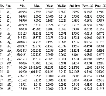
Table  2.   Descriptive Statistics

No. Var. Min. Max. Mean Median Std. Dev. Perc. - 25 Perc. - 75

1 R_i1 ­0.9954 9.8966 0.8463 0.5880 0.9999 0.1667 1.2500

2 R_i2 ­0.9964 8.0000 0.4600 0.2419 0.7506 ­0.0151 0.7500

3 R_i3 ­0.9966 9.0000 0.1627 0.0327 0.5932 ­0.1981 0.3689

4 R_i4 ­0.9939 6.6310 0.0528 ­0.0356 0.5175 ­0.2450 0.2186

5 X_it 0.0000 46.2025 0.2092 0.0968 0.9104 0.0532 0.1959

6 q_it ­55.1125 58.8148 0.0571 0.0071 1.7100 ­0.0313 0.0772

7 b_it ­54.3503 33.3750 ­0.0873 0.0011 1.7231 ­0.0608 0.0553

8 g_it ­10.6073 54.4328 0.1977 0.0683 1.2737 0.0056 0.1976

9 r_it ­29.9957 28.9790 ­0.1362 ­0.0737 1.3559 ­0.4694 0.0301

10 sr_it ­506.3845 202.6165 0.0336 0.0907 11.8351 ­0.1125 0.4198

11 lr_it ­250.0161 289.1262 0.2959 0.0609 6.3004 ­0.0368 0.2572

12 p_it ­54.3503 33.3750 ­0.0873 0.0011 1.7231 ­0.0608 0.0553

13 PB_it 0.0026 70.4000 1.0362 0.6831 2.4254 0.3594 1.2095

14 V_it 0.0100 6,843.3600 39.3251 3.6300 248.8796 1.1600 16.3400

15 B_it 0.0200 4,601.1500 29.8525 2.7450 189.1163 0.5400 10.6200

16 AR_i1 ­2.6632 8.9513 0.0000 ­0.2030 0.9306 ­0.5655 0.3361

17 AR_i2 ­2.3542 7.1236 0.0000 ­0.1283 0.6854 ­0.4069 0.2438

18 AR_i3 ­1.8951 8.5445 0.0000 ­0.0862 0.5433 ­0.3150 0.1953

[image:19.595.122.471.393.709.2]

19 AR_i4 ­1.3450 6.2174 0.0000 ­0.0818 0.4939 ­0.2785 0.1558

Table 1. Sample Data

Decrease Sample

No. Note Number % Number %

1 Population     24,095 100.00

2 Stock price data incomplete         8,939 37.10  15,156 62.90

3 Earnings data unavailable 661 2.74     14,495 60.16

4 Expected data unavailable 8,038 33.36       6,457 26.80

5 Lossing company exclusion 167 0.69       6,290 26.11

6 Extreme value exclusion 120 0.50       6,170 25.61

7 Inability to calculate abnormal return 38 0.16       6,132 25.45

This study performs data analysis to investigate initial data tendency. The descriptive statistics are  presented in Table  2.  Return  for  one  year  period (R_i1) is 0.8463, which then decreases over time and plunges to 0.0528 for R_i4. The decreases occur in all levels within 25th _{percentile (from 0.1667 to ­0.2450)}

and  75th  _{percentile  (from  1.2500  to}

0.2186). These findings indicate that market  value  in  the  longer  period  is closer  to  real  firm’s  intrinsic  value. With this tendency, the firm’s funda­ mental value calculated using account­ ing information is expected to be re­ flected in the firm’s market value.

Focusing on earnings after taxes (x_it),  this  study  only  employs  profit firms.  Earnings’  minimum  value  is 0.0000,  with  mean  0.2092,  median 0.0968, and standard deviation 0.9104. The  median  lies  on  the  left  from  its mean, signaling that some firms have extremely  great  earnings,  and  so  the mean is pushed upward. However, it is not a problem as the standard deviation is less than one. The aligned movement between  return  and  earnings  shows that they are likely to be related. The change  in  earnings  power  (q_it),  the change in growth opportunities (g_it), and long­run assets scalability (lr_it) show relatively the same pattern as the variation of earnings. Meanwhile, the change  in  discount  rate  (r_it),  the change in short­run assets scalability (sr_it), and the change in profitability (p_it)  show  otherwise.  However,  the change in discount rate is not expected to be aligned. Nevertheless, the change in short­run scalability and the change

in  profitability  with  such  movement may reduce the degree of association of the return model.

Firm’s book value (B_it), market to book value ratio (PB_it), and stock price (V_it) are always positive because, ac­ cording to the criteria, this study ex­ cludes  firms  with  negative  earnings after taxes and negative book values. Even after the elimination of extreme values, B_it and V_it still have large maxi­ mum  values,  especially  for  the  data from developing countries where stock market values usually move away from their book values. Book value (B_it) data with mean of 29.8525 and median of 2.7450 resemble the pattern of stock market  value.  The  pattern  does  not harm the  relation, and  the pattern  of firm’s intrinsic value (V_it) is reflected in stock  market value  at the  end of  ac­ counting period.

all  expected  values.  In  addition,  this study could achieve a higher degree of association.

Analysis of Chen and Zhang’s

(2003) Model

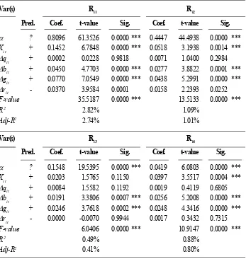
This  study,  at  the  first  analysis, examines  Chen  and  Zhang’s  (2003) model, which is the basic model (Model 12). The basic model constructs five cash­flow­related  factors  associated with return: (1) earnings yield (x_it), (2) the change in firm’s book value (b_it), (3) the change in earnings power (q_it), (4) the change in growth opportunities (g_it), and (5) the change in discount rate  (r_it).  The  results  of  the  first analysis are presented in Table 3.

The analysis of Chen and Zhang’s (2003) model has yet to examine this study’s hypotheses. Rather, it is con­ ducted as an initial investigation of the five cash­flow­related factors associ­ ated  with  stock  return.  The  results show that three variables, i.e., earnings yield (x_it), firm’s book value (b_it), and growth opportunities (g_it), are signifi­ cantly (at 1% level) related to various specifications  of  return  (R_i1  to R_i4). However, this study is unable to find evidence on the relation between earn­ ings  power  (q_it)  and  stock  return which  Chen  and  Zhang  (2003)  has proven  consistently.  Meanwhile,  the result for the change in pure  interest rate  (r_it),  as  in  Chen  and  Zhang’s (2003) model, is also insignificant. Con­

sequently, this study concludes that the basic  model  is  adequately  substanti­ ated, except for earnings power. How­ ever, the basic model analysis shows a sufficient degree of association with F­ value of 35.5187, which is significant at

1 percent level. The basic model has

R2 _{of 2.82 percent for R}

i1, and lower for other types of return. The degree of association with the  adjusted level is not significantly different, with adj-R2 of 2.74 percent_.

[image:22.595.127.474.176.542.2]

Table  3. The Results of Basic Model Analysis

Var(s) R_i1 R_i2

Pred. Coef. t-value Sig. Coef. t-value Sig.

 ? 0.8096 61.3526 0.0000 *** 0.4447 44.4938 0.0000 ***

X_it + 0.1452 6.7848 0.0000 *** 0.0518 3.1938 0.0014 ***

q_it + 0.0002 0.0228 0.9818 0.0071 1.0400 0.2984

b_it + 0.0450 4.7703 0.0000 *** 0.0277 3.8822 0.0001 ***

g_it + 0.0770 7.0549 0.0000 *** 0.0438 5.2991 0.0000 ***

r_it - 0.0370 3.9584 0.0001   0.0158 2.2393 0.0252  

F-value 35.5187 0.0000 *** 13.5133 0.0000 ***

R2 _{2.82%   1.09%}  

Adj-R2   _{2.74%       1.01%}    

Var(s) R_i3 R_i4

Pred. Coef. t-value Sig. Coef. t-value Sig.

 ? 0.1548 19.5395 0.0000 *** 0.0419 6.0803 0.0000 ***

X_it + 0.0203 1.5765 0.1150 0.0397 3.5517 0.0004 ***

q_it + 0.0084 1.5582 0.1192 0.0019 0.4119 0.6805

b_it + 0.0191 3.3806 0.0007 *** 0.0256 5.2008 0.0000 ***

g_it + 0.0246 3.7618 0.0002 *** 0.0248 4.3416 0.0000 ***

r_it - 0.0000 ­0.0070 0.9944   0.0017 0.3432 0.7315  

F-value 6.0406 0.0000 *** 10.9147 0.0000 ***

R2 _{0.49%   0.88%}  

Adj-R2   _{0.41%       0.80%}    

Notes: Number of observation (N): 6,132. Rit: stock return, firm i during period 1 (a year), 2 (a year and three months), 3 (a

year and six months), and 4 (a year and nine months); xit: earnings, firm i during period t; qit: change of profitability, firm

i during period t; bit: change of book value, firm i during period t; git: change of growth opportunities, firm i during period

t; rit: change of discount rate, firm i during period t; *** significant at 1% level, ** significant at 5% level, * significant

at 10% level. Linearity test for this model 12 shows that: (1) With Kolmogorov­Smirnov test shows t­value 9.036 and p­ value 0.000, and Jarque and Berra shows t­value 15,202.42 and chi­square 0.000, it means that the residuals are not distributed normally. However, normality test is ignorable for large data sample that is 6,132. It tends to follow a central limit theorem (Gudjarati 2003). (2) Glejser’s test  for heteroscedasticity shows that all variables have significance above 0.05, with t­value (sig.) xit amount to 0.013 (0.989); qit amount to ­0.014 (0.989); bit amount to ­0.007 (0.994); git amount

to ­0.073 (0.942); and rit amount to 0.010 (0.992). The test shows that the data is free from heteroscedasticity problem. (3)

Multicolinearity test shows that all variables have VIF about one which means that there is no colinearity among variables, VIF value for each variable is, xit amount to 2.394; qit amount to 1.483; bit amount to 1.664; git amount to 1.218; and rit

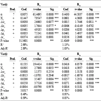
Analysis of Investment

Scalability Model

The  second  analysis  transforms the basic model analysis, in which we include the change in earnings power (q_it) into a model using the change in short­run  earnings  power  (sr_it)  and long­run earnings power (lr_it). This model is also called the short­run and long­run investment scalability induc­ ing model (Model 13). The model speci­ fies the earnings power into more de­ tailed forms to investigate their asso­ ciations  with  the  variation  of  stock price.  Table  4  presents  the  analysis results.

The results of Model 12 show that earnings yield (x_it), the change in book value  (b_it),  the  change  in  short­run earnings power (Dsr_it), the change in long­run  earnings  power  (lr_it),  the change in growth opportunities (g_it), and the change in discount rate (r_it) are associated with stock price move­ ment.  Consequently, H_A1, H_A4,  and

H_A5 are  confirmed  at  1  percent  level for  return  models R_i1 – R_i4. H_A4is partially supported at 10 percent level only for R_i1return type with t­value of 1.7644. H_{A3 is supported for R}

i1 return

type as well as for R_i2with t­value of 1.7466, which is significant at 10 per­ cent  level.  The  results  of  Model  13 examination show an adequate degree of association with F­value of 31.3601, which is significant at 1 percent level. The model has R2 _{of 2.98 percent for}

R_i1  type,  and  lower  for  other  return types. The model has adj-R2 _{of  2.89} percent.

The  analysis  results  show  that Model 13 is able to explain the relation between the change in earnings power (q_it) and stock return variation after specifying it into more detailed forms, i.e., short­run (sr_it) and long­run (lr_it) investment  scalabilities. H_A2 and H_A3

are  confirmed  for  both R_i1  and R_i2

return types. H_A2is also supported for

[image:24.595.123.473.170.523.2]

Table  4. The Results of Investment Scalability Model Analysis

Var(s) R_i1 R_i2

Pred. Coef. t-value Sig. Coef. t-value Sig.

 ? 0.8075 61.4695 0.0000 *** 0.4430 44.5037 0.0000 ***

X_it + 0.1447 7.9547 0.0000 *** 0.0601 4.3603 0.0000 ***

sr_it + 0.0030 2.6663 0.0077 *** 0.0015 1.7446 0.0811 *

lr_it + 0.0035 1.7644 0.0777 * ­0.0006 ­0.4149 0.6782

p_it + 0.0461 4.9185 0.0000 *** 0.0286 4.0283 0.0001 ***

g_it + 0.0833 7.5241 0.0000 *** 0.0461 5.4937 0.0000 ***

r_it ­ 0.0374 4.0118 0.0001   0.0156 2.2068 0.0274  

F­value 31.3601 0.0000 *** 11.6169 0.0000 ***

R2 _{2.98%   1.13%}  

Adj­R2   _{2.89%       1.03%}    

Var(s) R_i3 R_i4

Pred. Coef. t-value Sig. Coef. t-value Sig.

 ? 0.1535 19.4414 0.0000 *** 0.0416 6.0579 0.0000 ***

X_it + 0.0305 2.7868 0.0053 *** 0.0418 4.3937 0.0000 ***

sr_it + 0.0008 1.1375 0.2554 0.0008 1.3158 0.1883

lr_it + ­0.0013 ­1.0701 0.2846 ­0.0017 ­1.6076 0.1080

p_it + 0.0200 3.5407 0.0004 *** 0.0257 5.2351 0.0000 ***

g_it + 0.0250 3.7516 0.0002 *** 0.0271 4.6801 0.0000 ***

r_it ­ ­0.0004 ­0.0790 0.9370 0.0016 0.3181 0.7504

F­value 5.0317 0.0000 *** 9.7857 0.0000 ***

R2 _{0.49%   0.95%}  

Adj­R2   _{0.39%       0.85%}    

Notes: Number of observation (N): 6,132. Rit: stock return, firm i during period 1 (a year), 2 (a year and three months), 3 (a

year and six months), and 4 (a year and nine months); xit: earnings, firm i during period t; srit: change of short­run assets

scalability, firm i during period t; lrit: change of long­run assets scalability, firm i during period t; pit: change of

profitability, firm i during period t; git: change of growth opportunities, firm i during period t; rit: change of discount rate,

firm i during period t; *** significant at 1% level, ** significant at 5% level, * significant at 10% level. Linearity test for this model 13 shows that: (1) With Kolmogorov­Smirnov test shows t­value 9.035 and p­value 0.000, and Jarque and Berra shows t­value 15,202.42 and chi­square 0.000, it means that the residuals are not distributed normally. However, normality test is ignorable for large data sample that is 6,132. It tends to follow central limit theorem (Gudjarati 2003). (2) Glejser’s test  for heteroscedasticity shows that all variables have significance above 0.05, with t­value (sig.) xit amount to 0.045

(0.964); srit amount to ­0.045 (0.964); lrit amount to ­0.035 (0.972); pit amount to 0.000 (0.990); git amount to ­0.067

(0.946); and rit amount to 0.000 (0.990). The test shows that the data is free from heteroscedasticity problem. (3)

Multicolinearity test shows that all variables have VIF about one which means that there is no colinearity among variables, VIF value for each variable is, xit amount to 1.731; srit amount to 1.086; lritamount to 1.014; pit amount to 1.650; git

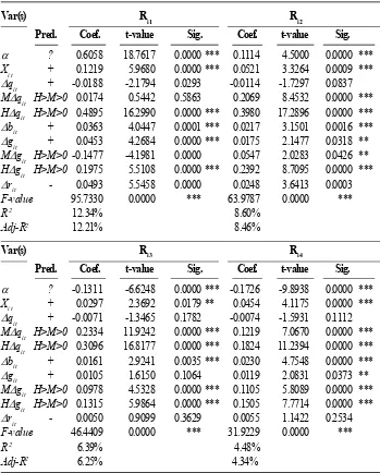
Sensitivity Analysis 1:

Categorical Arrangement

Subsequently, this study analyzes the model based on categorical differ­ entiation. This analysis serves to find a more favorable degree of association. Model 14 should have a higher good­ ness of fit when, after differentiation, it has a higher degree of association and is still  consistent with the main vari­ ables.  The  results  of  categorical  ar­ rangement  for  the  basic  model  are presented in Table 5.

This analysis purports to identify the  incremental  explanatory  power. Moreover, the categorical arrangement serves to identify the initial sensitivity such  that  hypotheses  examination  is supported  in  accordance  with  the theory.  The  categorical  arrangement for  Model  14  exhibits  that  there  are positive differences (greater than zero) for the changes in earnings power and growth opportunities. H_A1-H_A5 are ac­ cordingly supported, as are Model 13 above. In details, the change in earn­ ings power for high group (Hq_it) has a greater degree of association with t­ value of 16.2990, which is significant at

1 percent  level,  compared to  that  of

medium group (Hq_it). Similar results are applicable to growth opportunities. Model  14  shows  a  better  degree  of association with R2 _{of 12.34 percent}

and adj-R2  _{of  12.21 percent  for R}

i1 return type. Accordingly, Model 14 has been able to