T H E J O U R N A L O F H U M A N R E S O U R C E S • 45 • 3
The Needs of the Army
Using Compulsory Relocation in the Military
to Estimate the Effect of Air Pollutants on
Children’s Health
Adriana Lleras-Muney
A B S T R A C T
Recent research suggests that pollution has a large impact on asthma and other respiratory and cardiovascular conditions. But this relationship and its implications are not well understood. I use changes in location due to military transfers, which occur entirely to satisfy the needs of the army, to identify the causal impact of pollution on children’s respiratory hospitali-zations. I use individual-level data of military families and their depen-dents, matched at the zip code level with pollution data, for the period 1989–95. I find that for military children only ozone appears to have an adverse effect on health, although not for infants.
I. Introduction
One of the major justifications for pollution control is its potential effect on population health. The Clean Air Act states that its purpose is “to protect and enhance the quality of the Nation’s air resources so as to promote the public
Adriana Lleras-Muney is a professor of economics at UCLA. She thanks Mike Dove, Scott Seggerman, Tracee Matlock, and Edgar Zapanta at MDRC; David Lyle at West Point, Bryan Hubbell, Bonnie John-son, Jake Summers, David Lynch, and Terence Fitz-Simmons at the EPA; Jane Bomgardner at the FOIA office; and Marcia Castro at Princeton University for help in understanding spatial methods and using GIS software. She is very grateful to Joshua Angrist, Janet Currie, Angus Deaton, Rajeev Dehejia, Chrissy Eibner, Sherry Glied, Bo Honore´, Jeff Kling, Denise Mauzerall, Matt Neidell, Christina Paxson, and Jesse Rothstein for helpful discussions; to the seminar participants at Boston University, the Center for Health and Wellbeing and the Science, Technology and Environmental Program at Princeton Uni-versity, Cornell UniUni-versity, Vanderbilt UniUni-versity, Rutgers UniUni-versity, University of Maryland, University of California at Davis and the NBER summer institute for their comments; and to Nisreen Salti and Rebecca Lowry for outstanding research assistance. Funding from the National Institute on Aging, through Grant K12-AG00983 to the National Bureau of Economic Research, is gratefully acknowledged. These data were obtained through a Freedom of Information Act request. For further information please contact the author ⬍alleras@econ.ucla.edu⬎.
[Submitted April 2007; accepted February 2009]
550 The Journal of Human Resources
health and welfare and the productive capacity of its population.”1 But pollution
reductions are costly, thus for regulatory purposes it is important to determine the marginal external costs associated with polluting activities. Recent research suggests that pollution has a very large impact on asthma and other respiratory and cardio-vascular conditions (WHO 2003). But there is still much uncertainty about the mag-nitude of these effects. Using conventional data sets, it is difficult to separate the effects of pollution on health from the effects of socioeconomic background and of other characteristics of the areas where individuals live. Polluting factories locate in areas where land is cheap and constituents have low political leverage. High-pol-lution areas often have higher crime rates, fewer public services, and different av-erage socioeconomic characteristics. In addition, estimates of the effects of pollution can be biased because of sorting: Poor and disadvantaged families often live in polluted areas whereas wealthier (and healthier) families can afford to move to cleaner areas. On the other hand, individuals in worse health are more likely to move away from polluted areas (Coffey 2003).
I use changes in location due to military transfers to identify the impact of pol-lution on children’s health outcomes, measured by children’s hospitalizations. The military ordinarily requires that its members move to different locations in order to satisfy the needs of the army. These relocations are frequent, occurring every 24 to 48 months, and they affect all enlisted personnel and their families: about one-third of army families experience a Permanent Change of Station (PCS) in a given year. The military claims that within rank and occupation, all members are equally likely to be relocated to a particular base. If so, families are moved to high or low-pollution areas in a manner that is independent from their socioeconomic characteristics. I test the validity of this claim in various ways, and then use this unusual characteristic of Army families to obtain estimates of the effect of various pollutants on children’s health. I find that for military children only ozone appears to have an adverse effect on health, measured by respiratory hospitalizations. The effect is large: One standard deviation in O3increases the probability of a respiratory hospitalization by about 8– 23 percent.
Even if individuals were randomly assigned across locations, various character-istics of their environment other than pollution would be affected. Another important advantage of looking at military families is that, because they generally live on military bases, their living conditions remain relatively constant from base to base. Bases provide many services, including childcare, school, entertainment, and health-care (I discuss this in more detail below). Thus the variation in the environment (aside from weather and pollution) that military families experience when they move is small (relative to civilian families), so that unobserved neighborhood character-istics are not likely to be a large source of bias. Nevertheless, I perform several robustness checks to account for this possibility, including controlling for observed characteristics, adding base fixed effects, adding family fixed effects, and looking at the effects of pollution on hospitalizations for external causes. The results suggest omitted location characteristics are not problematic.
Lleras-Muney 551
There are other benefits to studying the effects of pollution using the military. First, there is no reason to suspect that the effects of pollution are different for military children than those for children in the general population. Second, all en-listed personnel and their dependents are covered by military health insurance (Champus/Tricare), which is quite generous (no premiums, low deductibles), and is highly rated by its members.2Therefore, issues of access to care are not first-order
concerns. Lastly, the data obtained from multiple administrative offices are very detailed and allow me to control for many potential confounders.
I focus on children because they are of particular interest. Lifetime (cumulative) exposure to pollution is close to contemporaneous exposure for young children—as children age, this is less true. Perhaps for this reason, children are suspected to be more susceptible than adults to pollution. Pollution is believed to cause various respiratory diseases and to aggravate existing respiratory conditions (for example, ozone and particulate matter are believed to precipitate asthma attacks).3Respiratory
diseases are the most common diseases among children and their economic costs are believed to be large,4especially because they are likely to be experienced over
a lifetime. Another advantage of focusing on young children is that their environment is less disrupted as a result of relocation, since they are not in school yet and most mothers of children younger than five in the military are at home.5
There is a vast literature in epidemiology that documents strong correlations be-tween pollution and mortality (for example, Pope et al. 2002; Samet et al. 2000), and between pollution and other health measures, including hospitalizations (WHO 2003). Two recent papers in economics (Chay and Greenstone 2003; Currie and Neidell 2005) look at the effects of pollution on infant mortality using plausibly exogenous time-series variation to identify the effects of pollution on infant mor-tality.6The identification strategy used in this paper uses cross-sectional and
time-series variation in pollution induced by relocations, and argues that, in the military, individual exposure to pollution is independent of individual- and site-specific char-acteristics. This identification strategy overcomes the two potential issues with these previous studies. One is that seasonal variation in pollution may be accompanied by changes in other variables that may affect health (for example, the decrease in pol-lution studied by Chay and Greenstone was induced by a recession, which most likely also lead to reductions in income and employment).
Another is that families may move as a result of high-pollution levels, especially if they suffer from respiratory problems. Although both studies (Chay and
Green-2. In 1995, 70 percent of spouses reported being satisfied with the Army Medical System. See footnote 9 for copay information.
3. Links to description of the sources and possible health consequences of each pollutant are found at: http://www.epa.gov/air/urbanair/6poll.html
552 The Journal of Human Resources
stone 2003; Currie and Neidell 2005) attempt to address the issue of omitted variable biases, neither addresses the issue of sorting. If, for example, sick individuals avoid polluted areas, this would mitigate the effect of pollution. Previous research indicates that avoidance behavior is important (for example, see Neidell 2009, or Neidell and Moretti 2008) and that individuals who experience health-related effects of pollution are more responsive than healthier individuals (Bresnahan, Dickie, and Gerking 1997). Coffey (2003) is the only study that specifically looks at the extent to which unhealthy households sort into areas with better air quality. He finds that there is indeed a substantial amount of sorting and his results suggest that sorting has a large impact on estimates of the effect of pollution on infant mortality. The design in this paper overcomes this sorting problem. In addition, this paper looks at hospitaliza-tions, which are a more frequent event than deaths.
This paper has a few limitations. Because I relate hospitalizations to annual pol-lution means, the effects here could be understated. The estimates here also can be downward biased because individuals avoid pollution, for example, by staying in-doors (Neidell 2009).
There are a number of additional contributions. I include measures for five major pollutants in the United States and find that models that look at the effects of a single pollutant at a time can be misleading. I use several methods to impute pol-lution at the zip code level and test the sensitivity of the models to distance from monitors. This is important because monitors are positioned generally in locations where pollution is suspected to be high. I find evidence that measurement error in pollution predictions is not classical and that it has large effects on the estimated coefficients.
The paper proceeds as follows. Section II describes the data used for the empirical analysis and a number of data-related issues. Section III describes the relocation process in the military and provides evidence that relocations cannot be predicted using individual characteristics of the enlisted men. Section IV presents the empirical strategy and the main results. In Section V concludes.
II. Data description and issues
A. Military personnel data
The data were provided by the Defense Manpower Data Center (DMDC) under the Freedom of Information Act. They contain annual individual-level information on enlisted married men and their dependents for the period 1988–98, including the characteristics of the enlisted men (age, race, education, occupation, rank, location, date of first enlistment, date of last enlistment, total number of months of active service7) and information on all hospitalizations (by condition) of their wives and
children. Individuals’ location is given by the zip code to which their sponsor (the
Lleras-Muney 553
enlisted father) is assigned to duty. Only information on individuals located in the Continental U.S. (48 contiguous states) was obtained. All characteristics are mea-sured as of December 31. (See section A of the Appendix available at www.econ.ucla/alleras).
B. Dependents’ health data
Military personnel and their dependents have access to care through two separate systems.8Military Treatment Facilities (MTFs) provide free care to all beneficiaries,
subject to capacity. Military families also obtain care through their health insurance known as Champus/Tricare. Under Champus (Civilian Health and Medical Program of the Uniformed Services), beneficiaries paid no premiums and were all subject to a single plan.9 Starting in 1995 a new system known as Tricare was phased in,
replacing Champus.
Generally beneficiaries are required to obtain care from an MTF if such care is available before using alternative care. The service area of an MTF generally in-cludes zip codes within 40 miles of the facility. In 1995 MTFs served about 89 percent of military dependents. Figure 1 shows the locations of all the military installations (most of which are bases) and MTFs for the Continental United States in 1990. Each circle represents an installation (the size of the circle is proportional to the number of observations) and each triangle represents an MTF.
Health data are obtained from the administrative claims filed by these two separate sources: MTFs and insurance. MTFs only filed claims for hospitalizations (no other services obtained at MTFs are observed).10 Champus/Tricare claims exist for
hos-pitalizations and for other services. Unfortunately Champus hospitalization claims do not report the diagnosis for the hospitalization (but most hospitalizations occur at MTFs—see below).
I construct several individual outcome measures using these claims. The first mea-sure is whether or not the person was hospitalized11during the year (regardless of
whether the hospitalization occurred in a military or private facility). Individuals with no hospitalization claims are assigned a zero. The second is whether the person was hospitalized in an MTF. For MTF hospitalizations only, I construct indicators for whether a hospitalization was for a respiratory condition (ICD9 codes 460 to 519, 769–770 and 786), an external cause (ICD9 800–999 or starting with “E”), or for any other cause. Births are not counted as hospitalizations. Infant mortality (or
8. Description and statistics come from Hosek et al. (1995) and Appendix X of the 1996 Department of Defense “Military Compensation Background Papers: Compensation Elements and Related Manpower Cost Items—Their Purposes and Legislative Backgrounds.”
9. The plan included small annual individual- and family-level deductibles ($100 per family if below E4 grade, $300 otherwise), a 25 percent co-pay for outpatient costs, and a $1,000 family stop loss. There was a daily nominal inpatient cost (not exceeding $25 annually in 1994).
10. Starting in 1996 the data from MTFs are no longer available. Because claims are reported in fiscal years (which begin in October), the data for MTF hospitalizations in 1995 is missing a quarter of that year’s hospitalizations, which would have been reported in 1996. Because of these changes, the data for 1995 are to be treated with caution.
554
The
Journal
of
Human
Resources
Figure 1
Distribution of military installations and military treatment facilities in 1990
Lleras-Muney 555
other health outcomes) cannot be constructed. Because hospitalizations are free, changes in income are unlikely to affect hospitalization rates.
C. Pollution and weather data
Pollution data come from the Environmental Protection Agency (EPA). They contain annual statistics for the period 1988–98 of measurements at the monitor level of the six major environmental pollutants in the United States, namely: particulate matter of ten micrometers in diameter (PM10), ozone (O3), lead (Pb), carbon monoxide (CO), sulfur dioxide (SO2), and nitrogen dioxide (NO2). Only monitors that appear
in at least eight years out of 11 are kept, and the missing values were interpolated within monitors over the years to obtain a balanced panel of monitors.12The final
number of monitors is reported in Section D of the Appendix available at www.econ.ucla/alleras.
Weather data (temperature, humidity and rain) from the National Climatic Center were also merged. For zip codes without measurements, temperature and rain were predicted in the same fashion as pollution (see next section and Section B of the Appendix, available at www.econ.ucla/alleras). Weather conditions are important potential confounders. For example, very hot weather during the summer raises O3 levels and also may result in more deaths. Weather also clearly changes with loca-tion. For this reason, I use both annual and quarterly measures to test the sensitivity of the results to detailed weather controls.
D. Assignment of pollution levels to individuals
For each individual in the data, we must estimate exposure to each pollutant using the pollution measurements obtained from monitors (located at a given longitude and latitude). This requires estimation of pollution levels for zip codes for which there are no monitors (the vast majority of zip codes). The simplest commonly used procedure is Inverse Distance Weighting (IDW), which assigns individuals the weighted average of pollution across monitors within a given radius, using the in-verse of the distance to the point as weights (as in Currie and Neidell 2005). Another simple option is to calculate county averages by averaging values across monitors in a given county (as in Chay and Greenstone 2003). Alternatively one can use Kriging. Kriging consists of estimating the parameters that describe the spatial cor-relation between observations and then using the estimates to find predictions that minimize the sum of squared errors.13Kriging predictions are based on the annual
12. The data provided by the EPA contain an unbalanced panel of monitors for each pollutant. In calcu-lating pollution levels for any given area, the addition and deletion of monitors are problematic if year-to-year variation within area is to be exploited. New monitors are usually added because the EPA learns of a source of emission. This generates a sharp increase in pollution from one year to the next at that location that isn’t necessarily real. Conversely, monitors are often removed because the area is compliant (pollution levels are low). Predictions for the area that are calculated using remaining adjacent monitors will over-estimate the pollution level.
556 The Journal of Human Resources
arithmetic mean at each monitor. The details of this method are given in Cressie (1993). Covariates may be used as well (in which case the method is referred to as co-Kriging) if there are other variables that are known to predict levels of pollution. These include annual measures of weather (rain, temperature, humidity, and wind direction), terrain (altitude), and emission sources (which are not available for this period and therefore not included). Today there are more sophisticated methods to map emissions into ambient concentration, using emission sources, topography, weather and other variables (for example, see Bayer, Keohane, and Timmins 2006) but the necessary data to estimate these models is unavailable for the period under study.14
Kriging has several advantages over the alternative methods previously used by economists (Cressie 1993). First, Kriging is the best linear unbiased predictor. Sec-ond, measures of fit of standard errors of the predictions can be obtained. Third, covariates can be used to improve the predictions. Lastly, Kriging allows prediction for a much larger number of locations in the United States compared to IDW or county averages.15
Research in geoscience suggests that Kriging methods are superior to deterministic methods theoretically and specifically for predicting pollution in the United States (Zimmerman et al. 1999, Anselin and Gallo 2006, Phillips et al 1997, and Hopkins et al. 1999). For example, Zimmerman et al. (1999) find using simulation methods that “Kriging methods were substantially superior to the inverse distance weighting methods over all levels of surface type, sampling pattern, noise, and correlation.” Kriging is also the methodology employed by the EPA to predict ozone and PM. They report that, “Support for these methods [specifically Kriging] has emerged from scientists and state/local/EPA agencies in recent workshops” (EPA 2004). Because of these advantages Kriging predictions are used for the main results.
Maps for the Kriging predictions for each pollutant for 1990 (see Section C of the Appendix available at www.econ.ucla/alleras) show that the highest (annual) concentrations of ozone were in California and the states in the Mid-Atlantic, East North Central, and South East regions. For PM10, the highest levels are found in California and Arizona. NO2 concentrations are highest in California and parts of
Texas. SO2concentrations on the other hand are lowest in California and highest in Pennsylvania and New York. CO is highest in the Northwestern and Eastern United States. These patterns are similar to those observed today. Overall pollution levels tend to be higher in urban areas, except for O3. There is a significant amount of
variation in pollution levels across the country, and this variation is different for each pollutant. Note that the predictions for Pb are poor (see Section D of the Appendix, available at www.econ.ucla/alleras).
I also match individuals to pollution levels computed using IDW (for both 15-and 30-mile radii) 15-and using county-level averages (where the weights are number of observations at each monitor in a given year). In all cases, individuals are matched
14. Additionally, these models are highly dependent on various assumptions and none is widely accepted in environmental sciences. For example, see Tong and Mauzerall (2006).
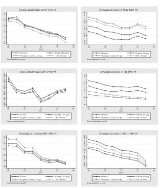
Lleras-Muney 557 Weighted County Average IDW, 30 miles Concentrations in ppm Weighted County Average IDW, 30 miles Concentrations in ppm Weighted County Average IDW, 30 miles Concentrations in ppm Weighted County Average IDW, 30 miles Concentrations in ug/m3 Weighted County Average IDW, 30 miles Concentrations in ug/m3 Weighted County Average IDW, 30 miles Concentrations in ppm
Unweighted trends in SO2 1988-95
Figure 2
Comparing trends from different prediction methods
to the predictions in the zip code to which their sponsor is assigned to duty. Figure 2 shows national trends (averages across zip codes) for all pollutants from 1988 to 1995 obtained using the various methods. All prediction methods yield trends that closely follow the trends obtained from monitor data. All pollutants show downward trends, with the exception of O3, which decreases until 1992, and starts rising
there-after.
558 The Journal of Human Resources
excellent predictions of outdoor pollution levels at the zip code level, because in-dividuals move around quite a bit. This problem is less likely to be an issue for young children in the military (compared to adults or children in the civilian popu-lation) since they live and go to school/daycare at the base or nearby. However, personal exposure will also depend on indoor pollution as well as on individual behavior (mobility and time spent outdoors). This is a limitation of using ambient pollution levels, which most studies use.16
Because military installations are generally located in rural (low density) areas, it is possible that the military’s exposure is not representative of the general population. To gauge this, I compute mean exposure for the population by averaging predictions over zip codes and using the population aged 18 and younger in the zip code as weights. (The population data come from the 1990 census STF 3A tapes.) I compare these averages with averages for military children 18 and younger in my data. Sec-tion E of the Appendix available at www.econ.ucla/alleras presents the means for both populations over the entire study period. The military are exposed to lower pollution levels on average, although the difference is generally small (less than half of a standard deviation) except for NO2.17 Different levels of pollution exposure
should not be of concern so long as the model used here to identify the effects of pollution on health is properly specified and there is overlap in the levels of pollution to which both groups are exposed. However, in the presence of nonlinearities (for which there is some evidence) the results may not easily be extrapolated to the population at large, limiting the external validity of this study (although external validity is a concern of most studies cited in the introduction as well.)
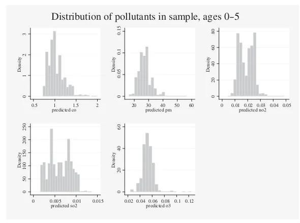
Figure 3 shows the distribution of pollutants for the final sample used in this study. The graphs document the variation in pollution that will often be used in the identification of pollution effects. Note that most pollutants have long, thin right tails—there are very few observations for the highest pollution levels. Previous re-search also has suggested that there can be strong correlations between different pollutants, generally because of common sources. For example, NO2, CO, and PM10 are all generated by automobile engines. Table 1 shows the correlations in my data. The largest correlation is about 0.5, between PM10 and CO. Also interestingly, there is a negative correlation between O3and CO.18
E. Sample and summary statistics
The hospitalization data show that about 11 percent of children were hospitalized at least once in the previous year. This hospitalization rate is higher than that observed for children of civilian parents but similar to what has been reported elsewhere for dependents of military personnel.19Most of these hospitalizations occur at an MTF.
16. Neidell (forthcoming) shows individuals respond to pollution alerts, biasing coefficients of the effects of ozone on health.
17. Section F of the Appendix available at www.econ.ucla/alleras shows the trends in exposure for both populations, which are also quite similar.
18. This has been observed in previous studies as well (for example, Samet et al. 2000). I also examined whether there is evidence of multicollinearity but found none.
Lleras-Muney 559
Distribution of pollutants in sample, ages 0-5
Figure 3
Table 1
Correlations between pollutants using Kriging estimates at the base
CO PM10 NO2 SO2 O3
SO2 0.0821 0.0684 0.2414 1
O3 ⳮ0.0208 0.228 0.1447 0.3593 1
SO2 0.2727 0.3377 0.4165 1
O3 ⳮ0.0307 0.1438 0.1438 0.2723 1
560 The Journal of Human Resources
0
0.
1
0.
2
0.
3
0.
4
0 5 10 15 20
Age
% hospitalized in MTF % hospitalized in MTF for respiratory % hospitalized
by age and type of hospitalization Percentage of children hospitalized
Figure 4
Among MTF hospitalizations (for which diagnosis codes are known), 26 percent are due to respiratory conditions. Figures 4 and 5 show the distribution of hospitaliza-tions for all ages. Hospitalization rates fall rapidly with age, bottoming out between aged five and 15, after which they start rising. Because hospitalization rates are so low for older children and since young children are more susceptible to the imme-diate effects of pollution, I limit the analysis to children younger than age five (but I test the robustness of the results to including other ages). Figure 5 suggests that children aged 0–1 exhibit a much larger rate of respiratory hospitalizations than children aged 2–5, so I analyze the effects of pollution separately for these two age groups.20
The sample includes observations from 1989 to 1995. There are no claims data from MTFs from 1996 forward. As DMDC recommended, the year 1988 is dropped because the health insurance claims data for that year appear to be incomplete. To minimize differences in access to care, individuals with no access to a military
differences in demographic characteristics and because of the very generous insurance provided by the military. Hosek et al. (1995) reported that “After correcting for demographic differences and other factors [...] the rates at which military beneficiaries used inpatient and outpatient services were on the order of 30 to 50 percent higher than those of civilians in fee-for-service plans.” They report that percentage of de-pendents that were hospitalized overnight was about 8.5 percent in the early 1990s (Table B.5) and ad-justing for covariates it is about 11.3 percent (Table 3).
Lleras-Muney 561
hospital are excluded. Also I exclude officers, since it appears that they may have a greater ability to affect relocations, and stepchildren—they are less likely to live and move with their enlisted father. Finally, I restrict the estimation sample only to those in bases for which the closest monitor is within 50 miles for all pollutants (I discuss this in more detail below). Individuals with missing explanatory variables were also dropped. The final sample includes 67,582 married enlisted men and 94,113 children. It includes roughly 3 percent of the Army any given year, and somewhat less for 1990 and 1991 because of deployments for the Gulf War (only children whose fathers are stationed in the continental United States are included).21
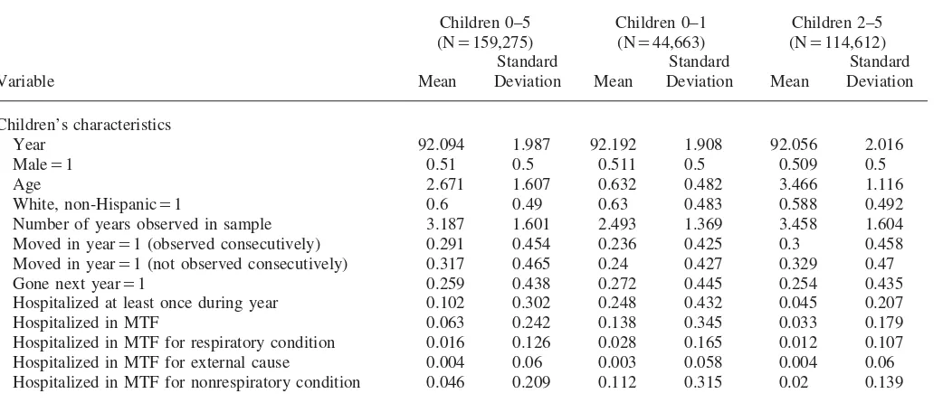
Table 2a shows the summary statistics for the sample. About half of the children are male, and 60 percent are white non-Hispanic. On average, children can be fol-lowed for 3.2 years (if no distance to monitor restriction is made). Of those who are observed in consecutive years, about 30 percent move—the same percentage reported by the military for the Army at large. The enlisted sponsors (dads) are about 29 years of age on average, have been on active duty for about nine years and have between two and three dependents (including their spouse); 12 percent have at least some college education. For those observed in two consecutive years,
562
The
Journal
of
Human
Resources
Table 2a
Summary Statistics for Children aged 0–5
Children 0–5 (N⳱159,275)
Children 0–1 (N⳱44,663)
Children 2–5 (N⳱114,612)
Variable Mean
Standard
Deviation Mean
Standard
Deviation Mean
Standard Deviation
Children’s characteristics
Year 92.094 1.987 92.192 1.908 92.056 2.016
Male⳱1 0.51 0.5 0.511 0.5 0.509 0.5
Age 2.671 1.607 0.632 0.482 3.466 1.116
Lleras-Muney
563
Father and mother characteristics
Number of dependents (including wife) 2.43 1.204 2.227 1.174 2.51 1.206 Some college or higher 0.118 0.323 0.102 0.303 0.124 0.33 Father’s age 29.259 5.283 27.566 5.241 29.919 5.151 Mother hospitalized at least once during year 0.202 0.401 0.362 0.481 0.139 0.346 Mother hospitalized in MTF 0.138 0.345 0.244 0.429 0.096 0.295 Mother hospitalized in MTF for pregnancy-related 0.108 0.31 0.223 0.416 0.063 0.242 Total active military service in months 106.497 61.969 87.629 60.435 113.85 60.996 Number of months since reenlistment 30.03 26.618 27.038 24.307 31.196 27.378 In the military fewer than six years⳱1 0.249 0.433 0.385 0.487 0.196 0.397 Increased rank (observed consecutively)⳱1 0.188 0.391 0.227 0.419 0.174 0.379
Increased education (observed consecutively)⳱1 0.021 0.143 0.019 0.136 0.022 0.145
564 The Journal of Human Resources
about 2 percent increase their education and about 19 percent move up in rank. For reference, the table also shows statistics separately by age.
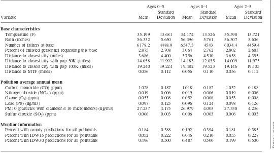
Table 2b shows the characteristics that are common in a base. There are 177 bases that appear in the study, although some of them are small and are not in the sample every year. Ultimately there are 935 base*year observations. The average base in the sample has about 6,100 married fathers, although there is a lot of variation across bases. Other base characteristics include distance to cities of varying size, distance to the closest MTF, and the number of Army personnel requesting that base in a given year as a first choice. These were collected to investigate the nature of relo-cations (see below). I report annual pollution means. I find that 18 percent of the sample has county predictions for all pollutants; 5 percent has IDW15 predictions for all pollutants, and IDW30 predictions exist for about 50 percent of the sample.
III. Describing relocations of military families
Military regulations require that enlisted personnel be relocated at least every three years, but no more than once a year. Moves are indeed frequent: Families are relocated every two and a half years on average, and every year about one-third of all military personnel make a permanent change of station (PCS). In a 20-year career, individuals are relocated an average of 12 times.22 Most soldiers
move their families as well: According to the 1987 Survey of Army families, 92 percent of the responding spouses said they were living in the same location as their spouse; in 1995, the percentage was 87.5 (Croan et al. 1992).
In principle, the army uses rank and military occupation (PMOS) in combination with “needs of the Army” to determine relocation. According to Army Regulation 614–200, “the primary goal of the enlisted personnel assignment system is to satisfy the personnel requirements of the Army. Secondary goals are to: (a) equalize desir-able and undesirdesir-able assignments by assigning the most eligible soldier from among those of like PMOS and grade; (b) equalize hardship of military service; (c) assign soldiers so they will have the greatest opportunities for professional development and promotion advancement; and (d) meet soldiers’ personal desires.”
The military unit responsible for relocation (previously known as Perscom) uses an automated system that produces target numbers by PMOS, rank, and location, and then constrains assignments to coincide with the targets. Generally, the needs (demand) in a given location within occupation and rank are driven by promotion, end of service, and retirement. Supply also is determined by these factors, and it is further constrained by regulations governing frequency of moves, training, enlist-ment, and base-closings, as well as by humanitarian considerations (see below).
Within these constraints, soldiers’ preferences may be taken into account. Soldiers submit up to three assignment preferences a few months before their next duty assignment. In practice enlisted personnel are generally not assigned to their pre-ferred location. Among those surveyed in 1987, only 35 percent reported that they were assigned to their preferred location (Burnam et al. 1992). Moreover these
Lleras-Muney
565
Table 2b
Summary Statistics for base level characteristics
Ages 0–5 Ages 0–1 Ages 2–5
Variable Mean
Standard
Deviation Mean
Standard
Deviation Mean
Standard Deviation
Base characteristics
Temperature (F) 35.199 13.681 34.174 13.526 35.598 13.721 Rain (inches) 56.332 5.650 56.396 5.761 56.307 5.606 Number of fathers at base 6178.2 4488.9 6547.3 4543 6034.4 4459.4 Percent of enlisted personnel requesting this base 2.875 2.708 3.064 2.762 2.802 2.683 Distance to closest city (miles) 3.686 4.400 3.756 4.510 3.658 4.355 Distance to closest city with pop 50K (miles) 14.058 11.992 14.183 12.035 14.009 11.975 Distance to closest city with pop 100K (miles) 19.240 19.224 19.482 19.523 19.146 19.105 Distance to MTF (miles) 0.056 0.112 0.056 0.110 0.056 0.112
Pollution average annual mean
Carbon monoxide (CO) (ppm) 1.028 0.187 1.018 0.182 1.032 0.188 Nitrogen dioxide (NO2) (ppm) 0.019 0.006 0.019 0.006 0.019 0.006
Ozone (O3) (ppm) 0.053 0.008 0.052 0.008 0.053 0.008
Lead (Pb) (ug/m3) 0.097 0.125 0.096 0.124 0.098 0.126 PM10 (particles with diameterⱕ10 micrometers) (ug/m3) 27.237 4.175 26.979 4.003 27.338 4.236 Sulfur dioxide (SO2) (ppm) 0.006 0.003 0.006 0.003 0.006 0.003
Monitor information
Percent with county predictions for all pollutants 0.184 0.388 0.192 0.394 0.181 0.385 Percent with IDW15 predictions for all pollutants 0.052 0.222 0.046 0.210 0.055 0.227 Percent with IDW30 predictions for all pollutants 0.496 0.500 0.487 0.500 0.499 0.500
566
The
Journal
of
Human
Resources
Table 2b (continued)
Ages 0–5 Ages 0–1 Ages 2–5
Variable Mean
Standard
Deviation Mean
Standard
Deviation Mean
Standard Deviation
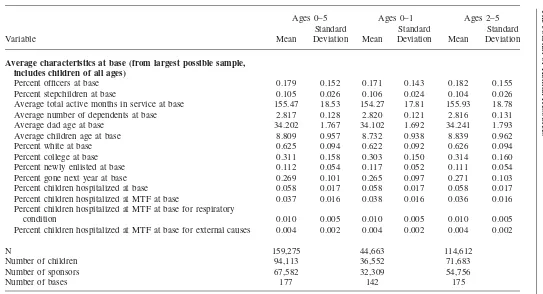
Average characteristics at base (from largest possible sample, includes children of all ages)
Percent officers at base 0.179 0.152 0.171 0.143 0.182 0.155 Percent stepchildren at base 0.105 0.026 0.106 0.024 0.104 0.026 Average total active months in service at base 155.47 18.53 154.27 17.81 155.93 18.78 Average number of dependents at base 2.817 0.128 2.820 0.121 2.816 0.131 Average dad age at base 34.202 1.767 34.102 1.692 34.241 1.793 Average children age at base 8.809 0.957 8.732 0.938 8.839 0.962 Percent white at base 0.625 0.094 0.622 0.092 0.626 0.094 Percent college at base 0.311 0.158 0.303 0.150 0.314 0.160 Percent newly enlisted at base 0.112 0.054 0.117 0.052 0.111 0.054 Percent gone next year at base 0.269 0.101 0.265 0.097 0.271 0.103 Percent children hospitalized at base 0.058 0.017 0.058 0.017 0.058 0.017 Percent children hospitalized at MTF at base 0.037 0.016 0.038 0.016 0.036 0.016 Percent children hospitalized at MTF at base for respiratory
condition 0.010 0.005 0.010 0.005 0.010 0.005 Percent children hospitalized at MTF at base for external causes 0.004 0.002 0.004 0.002 0.004 0.002
N 159,275 44,663 114,612
Number of children 94,113 36,552 71,683
Number of sponsors 67,582 32,309 54,756
Number of bases 177 142 175
Notes: ug/m3stands for micrograms per cubic meter; ppm stands for parts per million. Sample: children aged 0–5 of married men enlisted in the army and stationed in
Lleras-Muney 567
bers overestimate the amount of choice. Individuals learn (and the Army encourages them) to “play the system” by submitting preferences for locations where their skills are needed and where they can further develop their career.23 Thus the choices
soldiers list are constrained; for example, if an individual is due for an overseas transfer, he is unlikely to list a U.S. base among his choices, even if he does not want to go overseas.
This evidence is consistent with the idea that most individuals have very little choice over their relocations and that, within rank and occupation, assignment is not related to other individual characteristics of the enlisted personnel. Some individuals may nevertheless have more control over their relocations than others. According to Croan et al. (1992), junior ranking soldiers have the least control over where and when they move (also see Segal 1986). Because of this evidence I drop officers from my sample and focus on lower ranked soldiers. For this paper it is particularly important to know if relocations are correlated with family health, in particular children’s health. The army to some extent does consider family health needs in relocation assignments through the Exceptional Family Member Program (EFMP). The EFMP program is designed to be an assignment consideration and not an as-signment limitation.24EFMP only results in assignments to locations where needs
can be met if available, not to relocations that soldiers prefer. Of particular interest for this study is the fact that EFMP is not granted because of “Climatic conditions or a geographical area adversely affecting a family member’s health, [even if] the problem is of a recurring nature.”25
To further support the empirical strategy in this paper, I provide statistical evi-dence that individual characteristics observed at the time of relocation are uncorre-lated to base of relocation or to pollution levels at the new base. First, using the sample of individuals that are observed in different locations in two consecutive years, I estimateNequations of the form:
P
(
location⳱j)
⳱cⳭX (1) i,tⳭ1 i,t
Ⳮ
兺
␥i*I(
rank*occupation*year)
Ⳮεi,t,∀j⳱1,...Ni,t
These are linear probability models that predict the location of individualiin year
tⳭ1 based on individual characteristicsXin yeart(which include all of the spon-sor’s characteristics, mother’s hospitalization variables and, importantly, all of the child’s hospitalization variables) and a set of dummies for each rank, occupation, and year cell.26 The error terms are clustered at the sponsor level since a sponsor
can have several children and they may be observed in several years. There are as many equations as bases to which individuals are relocated. Among those who move
23. See regulation AR 614–200 3.3.
24. Governing regulation AR 608–75, dated May 1996.
25. This information is published online by the Air Force Personnel Center and is available at: http:// www.afpc.randolph.af.mil/efmp-humi/efmp-humi.htm. Although this paper looks at Army, not Air Force personnel, this information is indicative of Army practices in general.
568 The Journal of Human Resources
betweentandtⳭ1, no other observed characteristics other than rank and occupation in yeartshould predict location in yeartⳭ1. For each regression, I perform a joint test that⳱0. If, indeed, individual characteristics are orthogonal to location, then the vast majority of the tests should not reject the null.
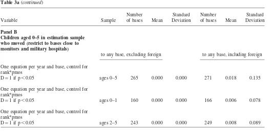
In Table 3a, I present the distribution of thep-values for these tests. In Panel A, I look at relocations to all bases (excluding foreign bases) from all bases for parents of children aged 0–5. In order to maximize the sample size for this test I do not drop individuals without access to MTFs or those in bases far from pollution moni-tors. Only in 6.6 percent of the regressions are individual characteristics predictive of relocation. If I include foreign bases this becomes 10.6 percent. Thus, at the 10 percent level we cannot reject the hypothesis that relocations are uncorrelated with observable characteristics beyond occupation and rank for relocations within the United States. In Panel B, I use only individuals included in the estimation sample, altogether or broken by age groups. Whether or not I include relocation to foreign bases, at the 5 percent level we cannot reject the hypotheses that individual char-acteristics are orthogonal to location.27
This evidence suggests that for the vast majority of enlisted personnel, relocations are not chosen. A weaker but relevant test is whether personal characteristics (in particular health or SES) predict pollution at relocation bases. For example, are high SES sponsors more likely to request bases that have low-pollution levels? This would appear not to be the case. In interviews, bases located closer to cities were generally preferred, and they tend to be more polluted on average. Some bases are universally thought of as undesirable, mostly for their remoteness and weather conditions, and due to the lack of availability of some services such as good schools. On the other hand, these same rural bases can be desirable from a career perspective because of the training opportunities available. (Fort Polk is a frequently cited example.) A priori this anecdotal evidence suggests that even if individuals were able to choose their location, it is not clear how their characteristics would be correlated to pollu-tion. But to test this in the data I estimate the following equations:
Y ⳱cⳭX Ⳮ ␥*I
(
rank*occupation*year)
Ⳮε ,(2) i,tⳭ1 i,t
兺
i i,t i,twhere Y is the pollution level that individual i is exposed to in yeartⳭ1, and X
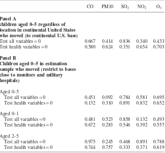
includes all of the same individual characteristics mentioned above in year t, in-cluding yeart’s hospitalization variables for mother and child. I estimate one equa-tion per pollutant. Again the sample is restricted to those that move between two years. The errors are clustered at the base level. For each equation I test whether the Xs are jointly significant, and also whether the health variables are jointly sig-nificant. The results are presented in Table 3b. In Panel A, I use the largest sample of 0–5-year-olds that moves bases. In Panel B, I present results for those in the estimation sample who moved. In all cases, the test does not reject the null that the
Xs are not significant. Hospitalizations in yeart are also not significant predictors of pollution in yeartⳭ1 among movers.
Lleras-Muney
569
Table 3a
Testing whether individual and family characteristics at timetpredict location at timetⳭ1, conditional on rank and occupation interactions. Sample: Children aged 0–5 who moved
Variable Sample
Number
of bases Mean
Standard Deviation
Number
of bases Mean
Standard Deviation
Panel A
Children aged 0–5 regardless of location in continental United States who moved
to any base, excluding foreign to any base, including foreign
One equation per year and base, control for rank*pmos
D⳱1 if p⬍0.05 ages 0–5 380 0.066 0.248 386 0.106 0.309
570
The
Journal
of
Human
Resources
Table 3a(continued)
Variable Sample
Number
of bases Mean
Standard Deviation
Number
of bases Mean
Standard Deviation
Panel B
Children aged 0–5 in estimation sample who moved (restrict to bases close to monitors and military hospitals)
to any base, excluding foreign to any base, including foreign
One equation per year and base, control for rank*pmos
D⳱1 if p⬍0.05 ages 0–5 265 0.000 0.000 271 0.018 0.135
One equation per year and base, control for rank*pmos
D⳱1 if p⬍0.05 ages 0–1 160 0.000 0.000 166 0.006 0.078
One equation per year and base, control for rank*pmos
D⳱1 if p⬍0.05 ages 2–5 243 0.000 0.000 249 0.008 0.089
Lleras-Muney 571
Table 3b
Testing whether individual and family characteristics at timetpredict pollution levels at timetⳭ1. Sample: Children aged 0–5 who moved. P-values reported
CO PM10 SO2 NO2 O3
Panel A
children aged 0–5 regardless of location in continental United States who moved (to continental U.S. base)
Test all variables⳱0 0.667 0.414 0.836 0.340 0.433
Test health variables⳱0 0.580 0.624 0.351 0.654 0.703
Panel B
Children aged 0–5 in estimation sample who moved (restrict to bases close to monitors and military hospitals)
Aged 0–5
Test all variables⳱0 0.451 0.092 0.784 0.581 0.695
Test health variables⳱0 0.132 0.310 0.891 0.832 0.652
Aged 0–1
Test all variables⳱0 0.481 0.523 0.858 0.132 0.493
Test health variables⳱0 0.672 0.283 0.546 0.392 0.557
Aged 2–5
Test all variables⳱0 0.975 0.245 0.468 0.891 0.788
Test health variables⳱0 0.744 0.757 0.333 0.371 0.619
Linear regression models. Errors clustered at the base level. Individual and family characteristics tested include age, gender, health variables (whether hospitalized, hospitalized in MTF, hospitalized in MTF for respiratory condition), father/sponsor’s controls (number of months since last enlistment, total active months in the military, age, white, college degree, number of dependents, enlisted in the last five years), and mother’s health (whether hospitalized, hospitalized in MTF, hospitalized for pregnancy-related). The table tests whether all the individual and family explanatory variables (with the exception of the rank*occupation*year interactions) are jointly significant using anF-test.
572 The Journal of Human Resources
IV. Main results
A. Empirical approach
For each age group (aged 0–1 and 2–5), I estimate the following individual-level linear probability model,28
Hosp ⳱cⳭP ⳭX ⳭZ ␦Ⳮ ␥*I
(
rank*occupation*year)
Ⳮε ,(3) ibt bt ibt bt
兺
ibt ibtwhere the dependent variable Hospis a dummy variable indicating whether or not childiliving in basebwas hospitalized in yeartfor a respiratory condition;Xis a matrix that includes age, race and gender of the child, and ␥sare the coefficients for each possible rank*occupation*year cell. Z is a matrix of base-level character-istics, which always includes base fixed effects to minimize concerns of location-specific time invariant omitted variables. Because weather is a potential confounder, rain, temperature, and temperature-squared are included in all models. The main results in the paper include individual measures of pollution, rather than constructing an index for pollution because (a) pollutants are regulated individually, and therefore it is important to know the externalities associated with each; (b) it is not theoreti-cally clear how to create and interpret such an index (see Greene 1997 for a dis-cussion); and (c) there are potentially interactions between pollutants. However, in the next section I also report results using various indexes.
The coefficients of interest are the estimated s, which represent the effect of a given pollutant P on the probability the child was hospitalized during the year. Unbiased estimates can be obtained under the assumption that, conditional on the included covariates, there are not unobserved individual- or base-level characteristics that predict respiratory hospitalizations and are correlated with pollution.
If location is indeed not chosen and pollution is uncorrelated to own character-istics, then cross-sectional estimates of the effects of pollution will be unbiased. Adding individual characteristics or family fixed effects should not affect the esti-mates. Importantly, among individual characteristics I can control for whether the child was hospitalized for an external cause (which mostly include accidents and violence-related episodes).
In principle, one of the advantages of the military is that their lifestyle will remain relatively stable as they move across the country. Relocations are not systematically associated with promotions. The military adjusts compensation for differences in the cost of living across location (Title 37 Chapter 7 Section 403b United States code). Its insurance program during this period did not charge differential prices by loca-tion. The Army provides housing in several bases. It also attempts to guarantee the availability of a number of services across all military bases, both to enlisted per-sonnel and their families, including counseling, relocation assistance, fitness facili-ties, libraries and recreation centers, among others. It is difficult to ascertain the extent to which the number and quality of these programs vary across locations.29
28. Results from logits are similar to those presented here.
Lleras-Muney 573
But according to some, “the Army replicates the same plans at each base and does not take local conditions under consideration” (Way-Smith et al 1994, quoted in Buddin 1998).
However there may be characteristics of the location that vary with pollution and also affect health, such as proximity to an urban area. In order to separate the effects of pollutants from those of other base characteristics, I take several approaches. In addition to base fixed effects, I add controls for a number of base- and year-level characteristics, including the percentage of sponsors that requested that base that year and the percentage of children that were hospitalized for external causes. This last variable should control for other base characteristics like crime. Lead also is included as a base level control, although the predictions for lead are fairly poor. Because weather is an important confounder that varies across bases and potentially affects health and pollution levels, I repeat estimation using quarterly rather than annual weather measures.
The specifications used here relate annual pollution measures to annual hospital-ization measures. Thus they measure the effects of pollution that occur within a relatively short period of time. However, previous studies have found effects of pollution within a year and even for much shorter windows (daily or weekly).30On
the other hand, the effects of pollution may be lagged or even cumulative over the years—these cannot be estimated here.
In all estimations the errors are clustered at the base level, since all individuals in the same base are exposed to the same levels of predicted pollution, which are measured with error and are likely to be correlated over time within bases (Bertrand et al. 2004).31
B. Main results
The results from estimating Equation 3 for each age group are presented in Tables 4a and 4b. All specifications include rank*occupation*year dummies. The first col-umn shows the effects of pollution when only age, gender, race, annual weather measures (temperature and rain), and base fixed effects are controlled for. The results for ages 0–1 show no significant effects, regardless of the specification in Table 4a. The pollutants are also insignificant when tested jointly (p-values for the test of joint significance are reported at the bottom of the table). I do not discuss results for this group in what follows.
The pattern is different for children aged 2–5. For them there appears to be a significant positive effect of O3. Column 2 adds all parental controls and a dummy for whether the child was hospitalized for an external cause. Again there is a sig-nificant positive effect of O3for children aged 2–5 similar in magnitude to that in Column 1. This is consistent with previous results that individual characteristics are uncorrelated with pollution levels at the base. Next, I examine the effect of
base-30. Chay and Greenstone (2003) relate annual infant mortality to annual pollution measures; Currie and Neidell (2005) look at mortality and pollution within a week; studies in epidemiology have commonly related daily mortality to levels of PM10 (for example, Samet et al. 2000).
574
The
Journal
of
Human
Resources
Table 4a
Effect of pollutants on respiratory hospitalizations, main results, children aged 0–1
(1) (2) (3) (4) (5) (6) (7)
Dependent variable: Child hospitalized last year for a respiratory condition (⳱1)
Basic controls
Parental controlsⳭ external hosp
Add base characteristics
Use quarterly measures of
rain and temperature
Family fixed effects
Movers (Family fixed
effects)
Nonmovers (Family fixed
effects)
Base FE Yes Yes Yes Yes Yes Yes Yes
Parental controls and
external hosp No Yes Yes Yes Yes Yes Yes
Base characteristics No No Yes Yes Yes Yes Yes Weather Annual Annual Annual Quarterly Quarterly Quarterly Quarterly
Lleras-Muney
575
CO 0.005 0.001 0 ⳮ0.009 0.034 0.173 0.013
[0.016] [0.016] [0.019] [0.023] [0.072] [0.206] [0.076] PM10 (*100) 0.064 0.039 0.04 0.056 ⳮ0.153 0.247 ⳮ0.205
[0.082] [0.078] [0.090] [0.083] [0.208] [1.243] [0.235] SO2 0.087 0.542 0.46 ⳮ1.049 ⳮ1.549 6.06 1.034
[1.537] [1.352] [1.571] [1.709] [5.629] [19.006] [6.236] NO2 1.087 0.42 ⳮ0.266 0.384 0.941 ⳮ3.38 1.539
[1.119] [1.162] [1.344] [1.253] [3.639] [23.619] [4.138] O3 ⳮ0.162 ⳮ0.182 ⳮ0.215 ⳮ0.141 ⳮ0.441 ⳮ0.186 ⳮ0.417
[0.320] [0.335] [0.288] [0.296] [0.791] [3.329] [0.915] Observations 44,663 44,663 44,663 44,663 44,663 5,971 38,692 R-squared 0.37 0.38 0.38 0.38 0.73 0.93 0.74
p-value (joint significance
of 5 pollutants) 0.414 0.8593 0.9543 0.9544 0.879 0.9476 0.9283
Basic regression controls for age dummies, female dummy, race dummy and pmos*rank*year interactions as well as rain, temperature and temperature squared. Family controls include number of months since last enlistment, total active months in the military, age, college degree, number of dependents, enlisted in the last five years, and a dummy for whether mother was hospitalized for pregnancy-related. Base characteristics include distance to closest city, distance to closest city with 50,000 inhabitants, distance to closest city with 100,000 inhabitants, distance to MTF, dummies for whether closest monitor is within 30 miles, number of sponsors at the base, percent of sponsors that requested base for relocation, Pb, percent officer, percent stepchildren, average number of months in service, average number of dependents, mean ages of sponsors at base, mean age of children at base, percent White non-Hispanic at base, percent of sponsors with some college, percent enlisted within the last five years, percent gone in the next year, percent of children hospitalized for external causes. Standard errors (in parenthesis) are clustered at the base level.
576
The
Journal
of
Human
Resources
Table 4b
Effect of pollutants on respiratory hospitalizations, main results, children aged 2–5
(1) (2) (3) (4) (5) (6) (7)
Dependent variable: Child hospitalized last year for a respiratory condition (⳱1)
Basic controls
Parental controls and
external hospitalizations
Add base characteristics
Use quarterly measures of
rain and temperature
Family fixed effects
Movers (Family fixed effects)
Nonmovers (Family fixed effects)
Base fixed effects Yes Yes Yes Yes Yes Yes Yes Parental controls and
external hosp No Yes Yes Yes Yes Yes Yes
Lleras-Muney
577
CO 0.007 0.007 0.008 0.002 0.024** 0.006 0.025*
[0.006] [0.006] [0.006] [0.008] [0.011] [0.037] [0.013] PM10 (*100) 0.008 0.007 0.014 0.026 ⳮ0.007 0.139 ⳮ0.001
[0.023] [0.023] [0.021] [0.029] [0.047] [0.149] [0.048] SO2 0.299 0.315 0.202 0.271 0.239 0.492 0.089
[0.566] [0.560] [0.544] [0.492] [1.117] [2.607] [1.163] NO2 0.32 0.318 0.081 ⳮ0.055 ⳮ0.353 ⳮ1.958 0.185
[0.385] [0.381] [0.297] [0.357] [0.567] [1.220] [0.729] O3 0.203* 0.200* 0.244** 0.207** 0.350** 0.129 0.351**
[0.104] [0.104] [0.100] [0.104] [0.154] [0.624] [0.172] Observations 114,612 114,612 114,612 114,612 114,612 21,428 93,184
R-squared 0.28 0.28 0.28 0.28 0.5 0.72 0.53
p-value (joint significance
of five pollutants) 0.2174 0.2214 0.0717 0.2177 0.0118 0.6444 0.0146
Basic regression controls for age dummies, female dummy, race dummy, and pmos*rank*year interactions as well as rain, temperature and temperature squared. Family controls include number of months since last enlistment, total active months in the military, age, college degree, number of dependents, enlisted in the last five years, and a dummy for whether mother was hospitalized for pregnancy-related. Base characteristics include distance to closest city, distance to closest city with 50,000 inhabitants, distance to closest city with 100,000 inhabitants, distance to MTF, dummies for whether closest monitor is within 30 miles, number of sponsors at the base, percent of sponsors that requested base for relocation, Pb, percent officer, percent stepchildren, average number of months in service, average number of dependents, mean ages of sponsors at base, mean age of children at base, percent White non-Hispanic at base, percent of sponsors with some college, percent enlisted within the last five years, percent gone in the next year, percent of children hospitalized for external causes. Standard errors (in parentheses) are clustered at the base level.
578 The Journal of Human Resources
level controls. Column 3 adds all base characteristics in addition to individual char-acteristics, and in Column 4, I replace annual weather measures with quarterly mea-sures. The effect of O3is positive and significant and remains around 0.2. All other coefficients remain insignificant.
In Column 5, I add family fixed effects. Pollution effects in this specification are identified by changes in pollution over time for those that remain in a given base, and due to changes in pollution associated with relocation for those that move. O3 remains positive and significant, although somewhat larger in magnitude. Interest-ingly, in these specifications CO is significant and larger than previously estimated. In Columns 6 and 7, I separate movers and nonmovers. For movers, the effects are identified from changes in pollution across bases only. The effect of O3 is not
significant and it is somewhat smaller, but not statistically different from the previous estimates. No coefficient is in fact significant in this specification, although it is worth noting that the sample size is greatly diminished. The results for nonmovers are very similar to those using the full sample: Both CO and O3 are positive and significant. It is perhaps surprising that the coefficients for movers are smaller than those for nonmovers. However, the mover sample uses observations before and after a move is observed. But the same individuals appear in the nonmover sample in those years when they do not move. So the samples contain the same individuals, but in different years. Since everyone is moved eventually, there is no one in the sample that is really a nonmover. Thus these results suggest that the effects of pollution are cumulative and thus are not observed in the short run (by definition in the mover sample exposure is short-possibly around six months, depending on the distribution of moves within calendar year, which is not known).
Across specifications, it also is worth noting that although insignificant, the effect of SO2 is always positive and relatively stable. The coefficient on NO2 is very unstable, and the effect of PM10 is also not very robust.
The results suggest that there are no statistically significant effects of pollution for children aged 0–1 on respiratory hospitalizations, and that O3(and perhaps CO but no other pollutant) significantly increases the probability of a respiratory hos-pitalization for children aged 2–5. Why would O3affect only older children? The
EPA suggests that “several groups are particularly sensitive to ozone—especially when they are active outdoors—because physical activity causes people to breathe faster and more deeply. Active children are the group at the highest risk from ozone exposure because they often spend a large fraction of the summer playing out-doors.”32Outdoor exposure most likely explains why there are no significant effects
of O3for children aged 0–1, since they are much less likely to play and exercise outdoors. These results are consistent with McConnell et al. (2002) who find that children that play sports and spend time outdoors are more likely to develop asthma only in areas with high ozone levels. In terms of magnitude the coefficient on O3, which ranges from 0.13 to 0.35, implies that an increase of one standard deviation in O3(0.008, 15 percent relative to the mean) increases the probability of a
respi-ratory hospitalization by 0.0010–0.0028 percentage points, or about 8–23 percent,
Lleras-Muney 579
relative to the mean for children aged 2–5 (0.012). The implied elasticity ranges from 0.5 to 1.5.
C. Specification checks and other estimation issues
Table 5 shows a number of additional specification checks for children aged 2–5 with all controls and quarterly weather and family fixed effects (as Column 5 of Table 4b). The first column reproduces the results from the previous table. In Col-umn 2 and 3, I test the sensitivity of the results to using different age groups. ColCol-umn 2 presents results pooling together all children aged 0–5. These results are very similar to those presented for children aged 2–5. Although as children age, they— like adults—may be less responsive to immediate changes in pollution, the age cutoff I chose for the main results is somewhat arbitrary. Thus, Column 3 present results for children aged 2–6 (results are similar but somewhat smaller if I include age seven as well). The effects of O3are robust to these changes, generally significant
and fluctuating between 0.1 and 0.3. The results for CO are qualitatively similar. Columns 4 and 5 test the sensitivity of the results to pollution outliers in the data. In Column 4, I drop observations where the value of any pollutant exceeds its 99th percentile or is below its first percentile. Figure 3 suggests that higher values rather than lower values of pollution may be problematic, so Column 5 drops all obser-vations where the value of the pollutant exceeds its 95th percentile for every pol-lutant. The results are somewhat sensitive to outliers. All the coefficients are insig-nificant, although both sample size and variation in pollution are diminished in these regressions. The effect of CO falls and is insignificant. The coefficient on O3is not
significant, and varies a lot in magnitude. These results suggest that outliers matter. In the last column, as a final way to assess whether omitted individual- and base-level characteristics are driving the results, I look at whether pollution predicts the probability that a child will be hospitalized for an external cause. In both panels, all of the coefficients for individual pollutants are statistically insignificant. They are also jointly insignificant.33
Table 6 compares the results obtained from different prediction methods and from limiting the sample based on distance to monitor. Again I present results only for children aged 2–5, with and without family fixed effects. The first column reproduces the results in Table 4b. In the next column, instead of adding all pollutants at once, I enter them one at a time. Because pollutants are correlated, and they can all potentially affect health, single-pollutant models (which are the most commonly used in the literature) can generate biased estimates of the effects of the pollutant in question. The effect of O3remains significant and is very similar whether it is entered alone or with other pollutants—perhaps this is to be expected since it is not strongly correlated with other pollutants. CO is also not very sensitive to adding other pol-lutants. But the effects of PM10, NO2, and SO2are quite sensitive to addition of other pollutants, even though these are insignificant.
Finally, I compare the results using Kriging to those obtained using inferior pre-diction methods used in previous research. In the next two columns I present the
580
Aged 2–5 Aged 0–5 Aged 2–6 Aged 2–5 Aged 2–5 Aged 2–5
Dependent
CO 0.024** 0.028*** 0.024*** 0.011 0.004 ⳮ0.003 [0.011] [0.011] [0.008] [0.013] [0.014] [0.016] PM10 (*100) ⳮ0.007 ⳮ0.021 ⳮ0.024 ⳮ0.004 0.017 ⳮ0.017 [0.047] [0.039] [0.036] [0.056] [0.064] [0.060]
SO2 0.239 ⳮ0.154 0.411 0.837 0.093 0.054
[1.117] [0.822] [0.951] [1.237] [0.899] [1.539] NO2 ⳮ0.353 0.19 ⳮ0.36 ⳮ0.194 ⳮ0.432 ⳮ0.316
[0.567] [0.517] [0.364] [0.686] [0.670] [0.650] O3 0.350** 0.310** 0.305** 0.092 0.611 ⳮ0.019
[0.154] [0.151] [0.123] [0.402] [0.440] [0.245] Obs 114612 159275 140666 100466 95456 114612
R-2 0.5 0.46 0.46 0.52 0.53 0.51
See notes in Table 4.
Lleras-Muney
581
Table 6
Comparing results from alternative predictions
Dependent variable: Child hospitalized in last year for respiratory condition (⳱1)
Monitors within 50 miles for all pollutantsa
Monitors within 30 miles for all pollutants
Monitors within 15 miles for all pollutants
At least one monitor in country for all pollutants
All at once One at a
time IDW 30
(co)
Kriging IDW15
(co) Kriging
County weighted
average
(co) Kriging
All controls
CO 0.002 0.004 0.004 ⳮ0.003 0.007 ⳮ0.029 ⳮ0.003 0.009 [0.008] [0.008] [0.007] [0.013] [0.026] [0.030] [0.007] [0.014] PM10 (*100) 0.026 0.03 ⳮ0.049* ⳮ0.021 0.022 0.057 0.01 0.025
[0.029] [0.029] [0.027] [0.042] [0.151] [0.218] [0.054] [0.107] SO2 0.271 0.545 0.745 ⳮ0.005 ⳮ3.887 ⳮ2.06 ⳮ0.112 1.459
[0.492] [0.465] [0.934] [1.168] [3.349] [3.763] [1.132] [1.637] NO2 ⳮ0.055 ⳮ0.003 ⳮ0.345 0.043 ⳮ0.435 ⳮ0.747 ⳮ1.137*** ⳮ0.141
[0.357] [0.337] [0.446] [0.538] [1.243] [1.541] [0.370] [0.644] O3 0.207** 0.216** 0.072 0.182 ⳮ0.761 ⳮ0.499 ⳮ0.299 0.379
[0.104] [0.104] [0.229] [0.120] [0.524] [0.518] [0.337] [0.263] Observations 114612 64348 64348 12103 12103 43353 43353
R-squared 0.28 0.36 0.36 0.58 0.58 0.37 0.37
582 [0.011] [0.011] [0.009] [0.012] [0.028] [0.035] [0.013] [0.019] PM10 (*100) ⳮ0.007 0.006 ⳮ0.093** ⳮ0.122** ⳮ0.045 ⳮ0.051 ⳮ0.02 ⳮ0.039 [0.047] [0.051] [0.044] [0.061] [0.110] [0.218] [0.067] [0.088] SO2 0.239 0.538 2.081** 0.619 1.297 3.873 0.904 1.787
[1.117] [1.186] [0.938] [1.737] [2.253] [2.393] [1.543] [1.877] NO2 ⳮ0.353 ⳮ0.352 ⳮ0.929 ⳮ0.562 ⳮ1.25 ⳮ1.391 ⳮ1.000* ⳮ0.993
[0.567] [0.607] [0.604] [0.574] [1.077] [1.133] [0.503] [0.678] O3 0.350** 0.367** 0.505 0.498** 0.005 ⳮ0.168 ⳮ0.482 0.097
[0.154] [0.153] [0.432] [0.215] [0.696] [0.548] [0.659] [0.363] Observations 114,612 64,348 64,348 12,103 12,103 43,353 43,353
R-squared 0.5 0.52 0.52 0.55 0.55 0.51 0.51
a. the sample includes bases for which the closest monitor for each of the five pollutants is within 50 miles of the base. All models include all controls as described in the notes for Table 4.