Full Terms & Conditions of access and use can be found at
http://www.tandfonline.com/action/journalInformation?journalCode=ubes20
Download by: [Universitas Maritim Raja Ali Haji] Date: 12 January 2016, At: 00:17
Journal of Business & Economic Statistics
ISSN: 0735-0015 (Print) 1537-2707 (Online) Journal homepage: http://www.tandfonline.com/loi/ubes20
The Quality Adjusted Price Index in the Pure
Characteristics Demand Model
Minjae Song
To cite this article: Minjae Song (2010) The Quality Adjusted Price Index in the Pure
Characteristics Demand Model, Journal of Business & Economic Statistics, 28:1, 190-199, DOI: 10.1198/jbes.2009.08032
To link to this article: http://dx.doi.org/10.1198/jbes.2009.08032
Published online: 01 Jan 2012.
Submit your article to this journal
Article views: 67
The Quality Adjusted Price Index in the Pure
Characteristics Demand Model
Minjae SONG
Simon Graduate School of Business, University of Rochester, Rochester, NY 14627 (minjae.song@simon.rochester.edu)
This paper computes a quality adjusted price index for the personal computer CPU from 1996 to 2000. The index is based on the pure characteristics demand model. I first compute the quality adjusted price index for the whole market, and show that it is very comparable with the hedonic price index but more sensitive to changes in product quality. Two types of the hedonic index are considered. One is the dummy variable index and the other is the formulation in Pakes (2003). When I group consumers by their willing-ness to pay for attribute improvement, the index shows consumer groups are differently affected by their product choices.
KEY WORDS: Consumer surplus; Discrete choice model of demand; New product.
1. INTRODUCTION
This paper computes a price index in the computer process-ing unit (CPU) market usprocess-ing the pure characteristics demand model (PCM hereafter) developed by Berry and Pakes (2007). The index is constructed using the compensating variation from an estimated utility function. The index constructed in this way is called the quality adjusted price index or the cost of living index (Trajtenberg1990; Nevo2003).
The quality adjusted price index has been computed for the CT scanner (Trajtenberg1990), the automobile (Pakes, Berry, and Levinsohn1993), and the ready-to-eat cereal (Nevo2003). However, all of these studies use the (random coefficient) logit demand model, which has the idiosyncratic logit error term in the utility function (Berry, Levinsohn, and Pakes1995).
In the PCM the compensating variation captures surplus changes solely related to product characteristics, and consumer heterogeneity and product choice are fully described by random coefficients on product characteristics.
I also compute the hedonic price index for comparison. I con-sider two types of the hedonic index. One is the dummy vari-able index that is based on coefficients on the time dummy variables in the hedonic regression (Griliches1971). The other is the formulation in Pakes (2003) (the Pakes index hereafter) that provides the upper bound on the quality adjusted price in-dex. Trajtenberg (1990) argues that the quality adjusted price index captures changes in product quality more accurately in any cases, while the use of the hedonic price index is justified for the case where quality changes result from process innova-tion.
Exploiting the advantage of having the estimated utility func-tion, I group consumers according to their willingness to pay for attribute improvement and compute the index for consumer subgroups. Consumers are heterogeneous in two aspects. First, they differ in their willingness to pay for quality improvement, mainly measured by the processing speed. Second, they differ in their valuations on capacity of extra data storage inside the processor (the level 2 cache).
The group index captures welfare changes that consumers experience from particular products that they purchase. For ex-ample, in a market with vertically differentiated products, con-sumers endowed with low values of the random coefficient buy
high-quality products. When new products of improved quality are introduced, they experience different price changes com-pared to consumers who buy low-quality products (i.e., those with high values of the random coefficient).
Using product-level data for the personal computer CPU from 1993 to 2000, I first compute the quality adjusted price index for the whole market in the one random coefficient PCM. The biggest decline occurs in the second and the third quar-ters of 1998 with 34% and 32.8% declines, respectively. These are periods when Intel, a dominant manufacturer of the CPU, slashed prices to recover its decreasing market share. The small-est decline occurs in the first quarter of 1999 and in the third quarter of 2000 with 1.4% and 6.7% declines, respectively. From the second quarter of 1999 to the second quarter of 2000, the index steadily decreases by 20%–28% thanks to a rapid in-crease in the processing speed and stable introductory prices for new products.
In the two random coefficient PCM the market index shows that consumers gain much more than in the one random coeffi-cient model when new products are introduced at the low end of the market. For example, in the first quarter of 1999, a half of new products were introduced at the low end of the market. While the index in the one random coefficient model declines by 1.4%, it declines by 41.2% in the two random coefficient model. This is because the one random coefficient model aver-ages out welfare gains from these new products.
The comparison with the hedonic price index shows that the two indices are very comparable, but also shows that the qual-ity adjusted price index is more sensitive to changes in product quality. Differences are prominent when new products are in-troduced, and when prices of existing products fall without new products being introduced.
The group index shows that price changes are significantly different across groups. For example, in the second and third quarter of 1998, periods with the biggest index declines, con-sumers who bought new products experienced more than a 40% decline, while consumers who bought the lowest quality
prod-© 2010American Statistical Association Journal of Business & Economic Statistics January 2010, Vol. 28, No. 1 DOI:10.1198/jbes.2009.08032
190
ucts experienced less than a 10% decline. The group index also shows that the larger price decline in the two random coefficient PCM in the first quarter of 1999 is driven by consumers at the low end of the market.
2. THE MODEL
2.1 Consumer Demand
Suppose I observet=1, . . . ,Tmarkets, and in each market there areNt consumers. Given market t,the indirect utility of
consumerifrom purchasing productjis
vtij=δijt−αipjt=xjtβi−αipjt+ξt+ △ξjt, for 1≤j≤J,
vti0=δ0t,
wherexjt is a vector of observable characteristics of product
j, βirepresents a marginal utility that consumeriderives from
product characteristics,pjt is the price of productj, andαi is
the individual-specific price coefficient.ξtis the mean utility of
unobservable characteristics at periodt,△ξjtis a detrended
un-observable characteristic withE(△ξjt)=0, andδ0t represents
the utility of choosing the outside option.
This demand model is called the pure characteristics demand model, since it does not have the additive idiosyncratic taste component (Berry and Pakes 2007). The simplest version of PCM is so called the vertical model in which there is only one random coefficient. In the vertical model consumers agree on product quality but differ in their willingness to pay for qual-ity improvement (Shaked and Sutton1982; Bresnahan 1987; Berry1994). The consumer consensus on the ranking imposes a substitution pattern that only products in the adjacent “neigh-borhood” are substitutes for each other. However, more ran-dom coefficients can be added to product attribute variables. With multiple random coefficients, the consensus on the prod-uct ranking does not hold any more, and a substitution pattern becomes more flexible.
As in all discrete choice models, the utility from the out-side option and the mean utility of unobserved characteristics cannot be separately identified without further assumptions. If the value of the outside option is assumed to be zero, that is, δ0t=0,for all periods, time dummy variables identify changes
in the mean value of unobservable characteristics over time. On the other hand, if the mean value of unobservable characteris-tics is assumed to be zero, that is,ξt=0,for all periods, then
the same time dummy variables identify changes in the utility from the outside option.
Pakes, Berry, and Levinsohn (1993) propose another identi-fying assumption that on average unobservable characteristics of continuing products do not change over time, where continu-ing products are defined as products that exist in both periods of
t−1 andt.Then, a change in the utility from the outside option can be identified from the mean difference between(δjt−δ0t)
and(δjt−1−δ0t−1)of those continuing products (see Song2007 for details).
2.2 Construction of the Quality Adjusted Price Index
The quality adjusted price index is computed using the com-pensating variation. For the discrete choice model, the
compen-sating variation (CV) for consumeriin periodtis defined as
CVit=
uti−uti−1
αi
,
whereuti=maxj(vtij)(Small and Rosen1981). One should note
that, since income effect is assumed away, there is no difference between the equivalence variation and the compensated varia-tion.
SummingCVit over all consumers, I obtain
CVt=
Assuming that changes in prices from periodt−1 tottake the formpjt=(1−µt)pt−1+ △pj(t−1), that is, the distribution of prices moves leftward by a factor of(1−µt)but the variance
remains the same, Trajtenberg (1990) shows that a quality ad-justed price index can be computed as
(1−µt)=
be interpreted as the reservation price that would make the con-sumer indifferent between the set of improved products in pe-riodtand the older set int−1. In other words, if the products intwere “offered at an average price of (1−1µ
t)pt+ε(for any
small ε >0), the consumer would prefer to have the older set instead” (Trajtenberg1990, p. 33).
Exploiting the structure of the utility function, I go one step further and construct the quality adjusted price indexes for con-sumer subgroups. Concon-sumers are grouped according to their values of random coefficients. Consumers with different val-ues of random coefficients make different consumption choices in each period. For example, if products are vertically differen-tiated so that the utility function with one random coefficient represents consumer preferences, that is,
vtij=δjt−αipjt=xjtβ−αipjt+ξt+ △ξjt, for 1≤j≤J,
vti0=δ0t,
a consumer with a low value ofαialways buys a higher quality,
or equivalently a more expensive, product than a consumer with a high value ofαi.As a result, these two types of consumers
experience different welfare changes over time, and the price index for each group reflects this difference.
In the case of the one random coefficient model, consumers can be divided into 10 groups if the 10 percentiles ofαiare
cho-sen, five groups if the 20 percentiles ofαiare chosen, and so on.
If the utility function has two random coefficients, consumers will be grouped along with two dimensions of their preferences, and divisions on each dimension are determined by values of each random coefficient.
Given a consumer groupIg,CVitis summed over consumers
belonging toIgto obtain
CVgt=CVt(i∈Ig)=
192 Journal of Business & Economic Statistics, January 2010
and the quality adjusted price index forIgis computed as
(1−µgt)=
PIgt
PIgt−1
, (1)
whereµgt=CVgt/(CVgt+pgt)withCVgt=CVgt/ng·pgtis the
average price of products that consumers in this group purchase in periodt.
It is not the unique feature of the PCM that consumers are grouped by values of random coefficients. In the random coef-ficient logit demand model (BLP), one can also construct the group index. However, the implication of this index is different due to the idiosyncratic logit error term. Consider BLP withαi
as the only random coefficient. There are two sources of con-sumer heterogeneity. One isαiand the other is the idiosyncratic
taste term (εijt) that is independent across consumers, products
and time.
There are two ways of grouping consumers in this case. The first way is to group consumers by the value of αi and
then draw iid random variables fromG(ε)to independently as-sign them to each consumer every period. However, this can be problematic as consumers in the same group can make totally different purchase decisions over time due to iid εijt. A
con-sumer who buys the most expensive product in period t may buy the least expensive one in periodt+1,and one may ques-tion implicaques-tions of this group index.
The second, maybe a more reasonable, way is to group con-sumers by the value of αi and compute the expected welfare
changes. However, all consumers have a nonzero probability of buying a given product. Therefore, impact of product entry/exit is not as significantly different across groups as in the PCM, so it is much less meaningful to construct the group index in the model with an idiosyncratic error term.
2.3 Comparison With Hedonic Price Index
I consider two types of the hedonic price index in compar-ison to the quality adjusted index. One is the dummy variable hedonic index and the other is the formulation in Pakes (2003). The dummy variable index refers to the index built from the time dummy variables in the hedonic regression. It is hard to link this index to the quality adjusted index due to its lack of a theoretical basis. In perfect competition coefficients in the he-donic regression represent the marginal cost of changing prod-uct characteristics, but in oligopolistic markets they also include markup. This makes it hard to predict their signs. Pakes (2003) discusses this problem in detail. Nevertheless, it is often used in markets where product characteristics significantly change over time. I present two specifications, one with price as the dependent variable and the other with the log of price as the dependent variable.
The Pakes index, on the other hand, provides an upper bound on the quality adjusted price index. Its main idea is to adjust income such that consumers can buy the same bundle available in a base period at prices of a comparing period. This income adjustment is an upper bound of true compensating variation. When product quality improves without significant increases in price, money is taken away until the consumer is moved back to a consumption bundle in the base period, and the amount taken is less than to move her to the base period utility level. So the Pakes index is supposed to be no higher than the quality adjusted index in an absolute term in this case.
Unfortunately, I cannot construct the exact Pakes index with my data set. To construct this index the price hyperplane should be estimated in the hedonic space for each period, but I do not have enough observations to do this. So I impose a constraining assumption that all periods share the same constant and error terms. This makes the estimated hyperplane less flexible than that of the Pakes index, but still allows me to apply it to my dataset. I call this index the constrained Pakes index.
In particular, I first run the hedonic regression with proces-sor speed and procesproces-sor speed interacted with the time dummy variables. The constant term and dummy variable for smaller level 2 cache are included but not interacted with the time dummy variables. The price hyperplane for periodtis estimated byht(ct)=Xtβt. When the log of price is used as the
depen-dent variable,ht(ct)=exp(Xtβt)exp(0.5σ2)whereσ2is a
con-sistent estimate of the variance of the error term. The average compensating variation for periodtis calculated as
sumption bundle of periodtat prices of periodt+1.
3. THE PRICE INDEX IN THE CPU MARKET
3.1 Estimates of the Demand System
The data used in estimation consists of price, quantity sold, and characteristics of products of Intel and AMD from the sec-ond quarter of 1993, the first period in which Intel introduced Pentium processors, to the third quarter of 2000. Main charac-teristics are the processing speed in mega hertz (MHz) and the capacity of the level 2 cache which is extra memory storage inside the processor. The level 2 cache enables the processor to speed up computation by reducing a communicating time between the processor and the main memory chip outside the processor. Usually Intel and AMD produce two sizes of the level 2 cache, and there is a significant price difference between the two types.
I use the second quarter of 1996 as the base period in re-porting all price indices. This is mainly to eliminate the role of 386 and 486 processors in comparing the quality adjusted index with the hedonic index. In that period Intel stopped producing 386 and 486 processors, and since then their market share re-mained under 5% until they disappeared in the third quarter of 1997. These processors are treated as the outside option in de-mand estimation due to no data on price. The quality adjusted price index is sensitive to this treatment as the utility of buying a product is in a relative term to that of choosing the outside option. The hedonic index is less sensitive as it only considers prices of products sold.
Table1shows market trends during the sample periods. First of all, product quality, measured by the processor speed, im-proved significantly. The first column shows that the (quantity weighted) average speed increased from 137 MHz to 701 MHz in less than five years. This is more than a 500% increase. The maximum speed rapidly increased in the late 1990s. The aver-age lifetime of the CPU was about eleven quarters before 1998,
Table 1. Market trend
Processor speed Price Quantity sold
Time Avg. speeda Change Avg. priceb Change Totalc Change
96Q2 137.0 100.0 327.3 100.0 16.2 100.0
96Q3 149.7 109.3 310.9 95.0 19.8 122.1
96Q4 157.1 114.7 334.9 102.3 23.0 142.1
97Q1 164.5 120.0 326.3 99.7 23.2 143.5
97Q2 189.1 138.0 400.7 122.4 20.9 129.1
97Q3 202.0 147.4 295.2 90.2 23.0 142.0
97Q4 213.6 155.9 278.3 85.0 23.1 142.9
98Q1 241.1 175.9 306.2 93.6 20.4 125.8
98Q2 293.3 214.1 373.6 114.1 20.5 126.4
98Q3 356.5 260.3 374.1 114.3 26.1 161.2
98Q4 372.5 271.9 287.1 87.7 30.7 189.5
99Q1 382.8 279.4 264.0 80.7 26.0 160.5
99Q2 427.8 312.2 255.8 78.2 23.7 146.6
99Q3 467.7 341.4 285.3 87.2 30.4 187.7
99Q4 526.1 384.0 297.2 90.8 37.7 232.8
00Q1 591.3 431.6 306.3 93.6 46.3 285.8
00Q2 645.1 470.8 286.9 87.6 50.1 309.1
00Q3 701.3 511.9 263.4 80.5 42.0 259.2
aThe quantity weighted average in mega hertz.
bThe quantity weighted average in U.S. dollars. cIn million units.
and shortened to five quarters afterwards with higher rates of product introduction and obsolescence.
Secondly, despite the drastic change in product quality, the price distribution in each period did not change signifi-cantly. The third and fourth columns in Table 1 shows that the (quantity-weighted) average price has declined slightly. The price of new products has been stable. The first Pentium Pro and the first Pentium II processors, introduced in 1995 and 1997, respectively, were marketed at higher than $1,000.00, but the subsequent new products were never priced at higher than $1,000.00.
Lastly, the last two columns of Table1 show that the mar-ket expanded. More consumers bought the CPU as its quality improved and price went down. There are a few periods where the total quantity went down compared to the previous period,
but the market expanded by about 260% in less than five years. This suggests that consumers prefer new products increasingly over time.
Considering all these trends, one may conclude that con-sumers are better off with improved and cheaper CPUs. How-ever, it is not trivial to measure how much they are better off with product quality changing drastically over time.
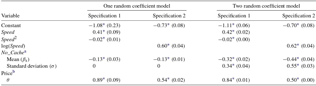
Table 2 shows estimates of the PCM. The estimation pro-cedure is explained in detail in Song (2007, 2008). Observ-able characteristics include the processor speed (Speed), the processor speed squared(Speed2)and the dummy variable for a smaller capacity of the level 2 cache(No_Cache)in the first specification, and the log of the processor speed [log(Speed)] and the dummy variable for a smaller capacity of the level 2 cache in the second specification. The dummy variables for
Table 2. Estimates of the pure characteristics demand model
One random coefficient model Two random coefficient model
Variable Specification 1 Specification 2 Specification 1 Specification 2
Constant −1.08∗(0.23) −0.73∗(0.08) −1.11∗(0.06) −0.70∗(0.08)
Speed 0.41∗(0.09) 0.42∗(0.02)
Speed2 −0.02∗(0.01) −0.02∗(0.00)
log(Speed) 0.60∗(0.04) 0.62∗(0.04)
No_Cachea
Mean (βs) −0.13∗(0.03) −0.13∗(0.01) −0.32∗(0.02) −0.44∗(0.04) Standard deviation(σ ) 0 0 0.34∗(0.04) 0.55∗(0.03) Priceb
θ 0.89∗(0.09) 0.54∗(0.02) 0.84∗(0.01) 0.50∗(0.00)
NOTE: Number of observations is 321. Dummy variables for quarters are included in all specifications. Standard errors are reported in parenthesis. aNo_Cacheis a dummy variable for processors with smaller capacity of the level 2 cache.
bThe price coefficient,α,is distributed log normal with mean set to zero; that is, log(α)∼N(0, θ ). ∗Significant at the 5% level.
194 Journal of Business & Economic Statistics, January 2010
quarters are included in all specifications, but are not reported in the table.
In the one random coefficient model, the random coeffi-cient is put on the price variable, and is assumed to be dis-tributed log normal with the location parameter fixed at 0, that is, log(α)∼N(0, θ1). This model imposes that consumers agree on the ranking of product quality but differ in their willingness to pay for quality improvement. In the two random coefficient model, another random coefficient is put on the dummy variable for a smaller level 2 cache, and is assumed to be distributed nor-mal, that is,βis∼N(βs, σ). In this model consumers evaluate
product quality in two aspects. One is whether a processor has a larger level 2 cache, and the other is the overall quality in terms of all other characteristics, mainly the processing speed.
Each model is estimated with two specifications. The first specification usesSpeed andSpeed2, and it shows that prod-uct quality is a concave function of the processor speed. Both
SpeedandSpeed2are significant at the 5% significance level. In the second specification, log(Speed)is used instead ofSpeed. By using the log, I restrict product quality to increase monoton-ically with the speed. log(Speed)is significant at the 5% level, and also shows that a higher processor speed is less appreciated over time.
In the two random coefficient model the average consumer is willing to pay $200∼$400 for putting the level 2 cache into the processor, while in the one random coefficient model the average consumer is willing to pay $80∼$110. The willing-ness to pay in the former model is more consistent with price differences between products of different sizes of the level 2 cache.
The variance of βis is significant, meaning that consumers
endowed with the sameαi value the level 2 cache differently.
The one random coefficient model does not reflect consumer heterogeneity on the level 2 cache by forcing products to be differentiated on the single dimension. Adding another random coefficient enriches the model by allowing consumers to be het-erogeneous in multidimensions. This difference between the two models will be more clearly demonstrated in the quality adjusted price index for different consumer groups.
As mentioned earlier, the coefficients on time dummy vari-ables capture a mixture of changes in the mean utility of unob-servable characteristics and in the value of the outside option. One cannot separate these two without assumptions. I use three different assumptions and compare results.
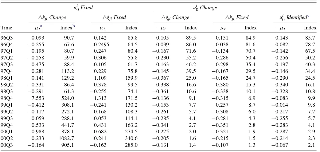
3.2 The Price Index for the Whole Market
I first compute the quality adjusted price index using the one random coefficient PCM. I use the first specification in Table2. Table3 lists price changes that the average consumer experi-ences (−µt) under different assumptions on the outside option
and unobservable characteristics. The average consumer is the one whoseαiis equal to the mean. The price index (PIt) is also
reported with the second quarter of 1996 as the base period.
−µtmultiplied by 100 gives a percentage change in price from
periodt−1 to periodtand
PIt=(1−µt)×PIt−1.
Following Nevo (2003), I first assume that the value of the outside option does not change over time (the columns labeled
ut0Fixed) and then assume that the mean value of unobservable characteristics (ξt) does not change over time (ut0Change).
Un-der the former assumption the time dummy variables identify
Table 3. The quality adjusted price index in the one random coefficient PCM
ut0Fixed ut0Change
△ξjtChange △ξjtFixed △ξjtChange △ξjtFixed ut0Identifiedc
Time −µta Indexb −µt Index −µt Index −µt Index −µt Index
96Q3 −0.093 90.7 −0.142 85.8 −0.105 89.5 −0.151 84.9 −0.143 85.7 96Q4 −0.255 67.6 −0.2495 64.5 −0.039 86.0 −0.038 81.6 −0.082 78.7 97Q1 0.195 80.7 0.247 80.4 −0.167 71.6 −0.134 70.7 −0.142 67.5 97Q2 −0.258 59.9 −0.306 55.8 −0.230 55.2 −0.286 50.4 −0.256 50.2 97Q3 0.475 88.4 0.105 61.7 −0.163 46.2 −0.298 35.4 −0.197 40.3 97Q4 0.281 113.2 0.229 75.8 −0.145 39.5 −0.167 29.5 −0.146 34.4 98Q1 0.141 129.2 1.109 159.9 −0.367 25.0 −0.165 24.7 −0.290 24.5 98Q2 −0.331 86.4 −0.378 99.5 −0.338 16.6 −0.380 15.3 −0.340 16.1 98Q3 −0.291 61.3 −0.255 74.1 −0.361 10.6 −0.338 10.1 −0.328 10.8 98Q4 7.553 524.0 1.313 171.5 −0.136 9.1 −0.315 6.9 −0.083 9.9 99Q1 −0.412 308.1 −0.241 130.2 −0.153 7.7 0.257 8.7 −0.014 9.8 99Q2 −0.117 272.1 −0.168 108.3 −0.261 5.7 −0.308 6.0 −0.217 7.7 99Q3 0.059 288.1 0.053 114.1 −0.285 4.1 −0.281 4.3 −0.255 5.7 99Q4 0.533 441.7 0.431 163.2 −0.341 2.7 −0.351 2.8 −0.283 4.1 00Q1 0.988 878.1 0.682 274.5 −0.275 2.0 −0.321 1.9 −0.287 2.9 00Q2 0.233 1082.7 0.241 340.6 −0.205 1.6 −0.215 1.5 −0.214 2.3 00Q3 −0.164 905.1 −0.163 285.0 −0.131 1.4 −0.107 1.3 −0.067 2.1
NOTE: The reported indexes are based on the first column in Table2.
a−µtmultiplied by 100 gives a percentage change in price from periodt−1 to periodt. bPI
t=(1−µt)PIt−1. 96Q2=100.
cThe value of the outside option is identified with the assumption that on average△ξjtof the continuing products does not change.
changes in the mean value of unobservable characteristics. Un-der the latter they identify changes in the value of the outside option.
For each assumption on the time effect I assume that un-observable characteristics change over time (△ξjtChange) and
that they do not (△ξjtFixed). In the former assumption all
resid-uals are interpreted as unobservable characteristics. The latter allows for measurement error in estimating product quality with a linear function of characteristics. In this case△ξjt is fixed at
the first period value for each product. Note that the motivation for the assumptions on△ξjtis not the same as in Nevo (2003).
The well-known problem of red bus and blue bus is not relevant to the PCM as it does not have an idiosyncratic taste term.
Table3shows that the index increases in about a half of time periods when the value of the outside option is fixed, and at the end of the sample period consumers become worse off. The as-sumption on△ξjt makes a significant difference so that change
in the compensating variation is much smaller when △ξjt is
fixed. However, the index still increases by more than two folds at the end of the sample period. The increased index is not sistent with the observed market trend. A larger number of con-sumers bought more improved products at lower prices in later periods. This contradiction suggests that the outside option im-proved over time. Consider a period from the third quarter of 1999 to the second quarter of 2000. This is a period where the (nominal) average price went up. The first two columns in the table show that consumers continued to be worse off during this period. This implies that quality improvement did not off-set price increase. However, if the outside option actually im-proved, quality improvement is underestimated.
On the other hand, the index continuously declines whenut0
changes over time, and it goes down below two at the end of the sample period. This is more consistent with the observed market trend. The index tends to go down further when△ξjtis
fixed. However, the assumption on△ξjtdoes not make a
signif-icant difference as much as whenut0is fixed.
In the columns labeledut0 Identified, the value of the out-side option is identified using the assumption that on average product quality of the continuing products does not change over time. Song (2007) uses this assumption and shows that the es-timated outside option increases and the mean of unobservable characteristics decreases in the late 1990s. The index is similar to whenξt is fixed (ut0Change), but declines less rapidly. That
is probably because the improvement in the outside option is exaggerated whenξtis fixed.
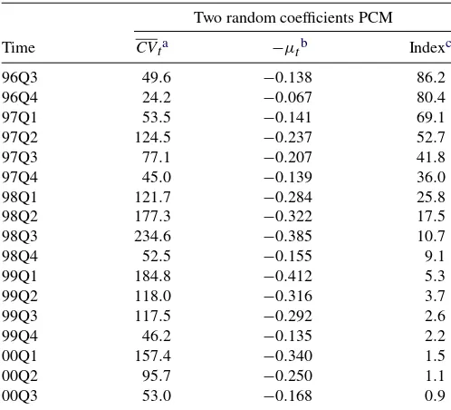
Table4lists the quality adjusted price index in the two ran-dom coefficient PCM. The value of the outside option is identi-fied using the same assumption as forut0Identifiedin Table3. The two indices are significantly different for periods after the third quarter of 1998. The index declines faster with two ran-dom coefficients so that it goes down to 0.9 at the end of the sample period. Most notably, in the first quarter of 1999 the in-dex declines by 41.2% in Table4, while it declines by 1.4% in Table3. This is the first period in which Celeron processors cap-tured considerable market shares. Although Celeron processors were first introduced in the third quarter of 1998, their market shares were tiny and only two Celeron processors were intro-duced. Moreover, one of two Celeron processors disappeared from the market in the last quarter of 1998. However, about
Table 4. The quality adjusted price index in the two random coefficient PCM
NOTE: The reported indexes are based on the third column in Table2. The value of the outside option is identified with the assumption that on average△ξjtof the continuing
products does not change. aIn U.S. dollars. b−µ
tmultiplied by 100 gives a percentage change in price from periodt−1 to periodt. cPI
t=(1−µt)PIt−1. 96Q2=100.
four out of 10 Intel processors are Celeron processors from the first quarter of 1999. The benefit consumers receive from these new products does not appear when products are ranked on a single dimension, but becomes significant with another random coefficient.
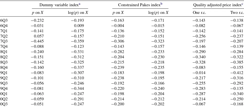
Table5reports the hedonic price index and compares it with the quality adjusted price index. The first two columns list the dummy variable hedonic index, and the third and fourth columns the constrained Pakes index. Each hedonic index has two specifications, one with price as the dependent variable and the other with the log of price. The dummy variable index uses processor speed, processor speed squared, the dummy variable for lower level 2 cache, and the time dummy variables as re-gressors. For the constrained Pakes index the processor speed and the processor speed squared variables are interacted with the time dummy variables. The last two columns list the quality adjusted price index for the one and the two random coefficient PCM.
The most significant difference between the dummy variable index and the Pakes index is their sensitivity to the economet-ric specification. The mean square difference between the two dummy variable indices is 0.038, while it is only 0.001 between the two Pakes indices. This suggests that the Pakes index is less prone to the specification error than the hedonic index. This is also consistent with Pakes (2003) who shows that his results are robust to various econometric specifications.
The comparison also shows that the second specification of the dummy variable index (the second column) is more similar to any of the Pakes indices than the first specification. Their squared mean difference is only 0.004, while it is about 2.3 with the first one. It also shows that the second specification of the dummy variable index tends to produce a higher number than
196 Journal of Business & Economic Statistics, January 2010
Table 5. Comparison with the hedonic price index
Dummy variable indexa Constrained Pakes indexb Quality adjusted price indexc
ponX log(p)onX ponX log(p)onX One r.c. Two r.c.
96Q3 −0.232 −0.193 −0.163 −0.171 −0.143 −0.138
96Q4 −0.031 0.009 −0.004 −0.015 −0.082 −0.067
97Q1 −0.141 −0.175 −0.136 −0.152 −0.142 −0.141
97Q2 0.057 −0.157 −0.210 −0.151 −0.256 −0.237
97Q3 −0.445 −0.359 −0.306 −0.323 −0.197 −0.207 97Q4 −0.088 −0.123 −0.143 −0.157 −0.146 −0.139 98Q1 −0.240 −0.331 −0.282 −0.233 −0.290 −0.284 98Q2 −0.151 −0.312 −0.204 −0.230 −0.340 −0.322 98Q3 −0.142 −0.325 −0.215 −0.218 −0.328 −0.385 98Q4 −0.160 −0.337 −0.239 −0.235 −0.083 −0.155 99Q1 −0.083 −0.307 −0.183 −0.198 −0.014 −0.412 99Q2 −0.101 −0.310 −0.238 −0.195 −0.217 −0.316 99Q3 −0.056 −0.246 −0.192 −0.166 −0.255 −0.292 99Q4 −0.081 −0.344 −0.220 −0.240 −0.283 −0.135 00Q1 −0.063 −0.247 −0.198 −0.204 −0.287 −0.340 00Q2 −0.059 −0.291 −0.214 −0.212 −0.214 −0.250 00Q3 −0.051 −0.247 −0.200 −0.202 −0.067 −0.168
aThe dummy variable index is calculated asPI
t=(γt−γt−1)/γt−1when the dependent variable is price andPIt=exp(γt−γt−1)−1 when the dependent variable is the log of price, whereγtis a coefficient on the dummy variable for periodt.pdenotes price andXdenotes product characteristics which include the constant term, speed, speed squared, and the dummy variable for smaller capacity of the level 2 cache. The time dummy variables are included in both specifications.
bThe constraining assumption is that all periods share the same constant and error terms. The index is constructed by−µt=CVt/(CV
t+pt)whereCVtis the upper bound of the
average compensating variation. See the text for howCVtis estimated.pdenotes price andXdenotes product characteristics which include the constant term, speed interacted with the
time dummy variables, speed squared interacted with the time dummy variables, and the dummy variable for smaller capacity of the level 2 cache. cThe value of the outside option is identified with the assumption that on average△ξ
jtof the continuing products does not change.
the Pakes index in an absolute term. It is true for all periods from the first quarter of 1998 to the end of the sample period.
It is hard to make an analytical comparison between the dummy variable index and the Pakes index due to the for-mer index’s lack of theoretical foundation, but my results give stronger support to the Pakes index. The dummy variable in-dex produces dramatically different numbers depending on the econometric specification, and it is not clear which specification should be chosen.
In the last two columns of the table, I list the quality ad-justed price index with the value of the outside option identi-fied. As explained earlier the Pakes index is supposed to be no higher than the quality adjusted index in an absolute term if both the utility function and the price hyperplane are precisely estimated.
The table shows that the quality adjusted index is almost al-ways higher in an absolute term. At least one of the quality adjusted indices is higher than both of the Pakes indices in 11 quarters out of 17. In eight quarters out of 11 quarters both of the quality adjusted indices are higher than both of the Pakes indices. In two quarters, the first quarter of 1997 and the fourth quarter of 1997, one of the quality adjusted indices is higher than one of the Pakes indices. Only in four quarters, both of the Pakes indices are higher than both of the quality adjusted indices.
A quarter-by-quarter comparison suggests that the quality ad-justed index gives more weight to quality changes, and this may be the main reason why the Pakes index is higher in some quar-ters. For example, in the third quarter of 1997 the quality ad-justed index goes down by about 20%, while the Pakes index goes down by about 30%. This is a period right after the in-troduction of the first Pentium II processor. This processor was
introduced at almost $2,000 and then its price dropped to below $1,000 in the next period. Comparing these two periods, the Pakes index declines much more in the third quarter of 1997, while the quality adjusted index declines more in the second quarter of 1997.
The fourth quarter of 1998 and the third quarter of 2000 are other examples. These are periods when no new product is in-troduced so there are no significant quality changes. In the first period the quality adjusted index goes down by about 10%, while the Pakes index declines by about 24%. In the second period the former index goes down by about 15%, while the latter declines by about 20%.
Pakes (2003) points out that one of the disadvantages of the Pakes index is that it is not necessarily close to the least upper bound of the compensating variation. My results show that its ratio to the quality adjusted index is about 0.70 on average, con-ditional on the former being lower than the latter. It is no lower than 0.61 and is as high as 0.75, depending on the specifica-tion. The period in which the two indices are the most different is the fourth quarter of 1996. The ratio is as low as 0.05 and no higher than 0.22. However, this period is clearly an outlier. Excluding this, the average ratio is no lower than 0.65 and as high as 0.82. The period with the two indices being the closest is the second quarter of 2000. The ratio is as high as 0.99 and no lower than 0.85.
3.3 The Price Index for Groups
In Table6 I report the quality adjusted price index for five consumer groups. They are grouped according to their values ofαi, where log(αi)∼N(0,0.89), so thatIjincludes consumers
whoseαi are in thejth quintile of the distribution. Consumers
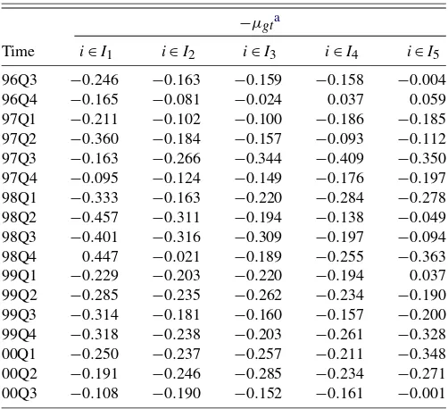
Table 6. The quality adjusted price index for groups
NOTE: The reported indexes are based on the first column in Table2. Consumers are grouped such thatIjincludes consumers whoseαiare in thejth quintile of the distribution.
The value of the outside option is identified with the assumption that on average△ξjtof
the continuing products does not change. a−µ
gtmultiplied by 100 gives a percentage change in price for groupgfrom period t−1 to periodt.
inI1 include those who buy the highest quality products and consumers inI5include those who buy the lowest quality prod-ucts and who do not buy any product. The value of the outside option is identified by the aforementioned way.
The table shows that each group experiences a different de-gree of price changes. For example, in the second and the third quarter of 1998 when the index for the whole market (the mar-ket index) falls by more than 30%, consumers inI1(the high end) experience more than a 40% drop, while those inI5(the low end) experience less than a 10% drop. This suggests that a large decline in the market index was caused by new product introduction at the high end of the market.
The table confirms that the introduction of 300 MHz Pen-tium II processor in the second quarter of 1997 benefits con-sumers considerably despite its high price. The index falls by 36% forI1in this period. However, in the third quarter of 1997 the index falls by only 16.3% for the same group despite an al-most 50% price decline. Considering the fact that no new prod-ucts were introduced in this period, this suggests that consumers benefit more from the quality improvement than from the price decline.
The table also confirms that the high-end market is responsi-ble for a modest decline in the market index in the fourth quarter of 1998, while the low-end market is responsible for a modest decline in the first quarter of 1999. In the former period con-sumers inI1 experience an increase in the index, while con-sumers in I5 experience a 36.3% decline. In the latter period consumers inI5experience an increase, while consumers inI1 experience a 22.9% decline.
In the third quarter of 2000 both the high and the low ends are responsible for a modest decline in the market index. Con-sumers inI1 experience a 10.8% decline and those in I5 ex-perience a 0.1% decline. A steady decline of the market index
from the second quarter of 1999 to the second quarter of 2000 is evenly contributed by all sectors of the market.
One should note that the presence ofξtin the utility function
may cause a problem in computing the group index.ξtmeasures
the mean value of unobservable characteristics of all products in periodt,and its value changes by both product entry/exit and changes in unobservable characteristics of continuing products. The following example shows how product entry/exit may dis-tort the group index in presence ofξt.
Suppose, as an extreme case, unobservable characteristics of individual products do not change over time once they are intro-duced in the market. Suppose further that no new products are introduced at the high end of the market in periodtand some products at the low end with relatively better unobservable char-acteristics exit the market at the end of periodt−1.For a group of consumers at the high end, the quality adjusted price index should merely depend on price changes. If this group buys the same products that they bought in period t−1 and prices do not change, the quality adjusted price index should not change either. However, sinceξt goes down due to the product exit at
the end of periodt−1,it will unjustly lower these consumers’ surplus, and so result in an increase in the price index.
The fourth quarter of 1998 is a good example. According to Table6, consumers at the high end experienced an increase in the index. This is a period where no new products were intro-duced and six products exited the market. Since unobservable characteristics of the continuing products are assumed not to change over time, an increase in the index means that nominal prices of existing products went up. However, prices of the high end products actually decreased. A real cause of the index in-crease may come from a dein-crease inξt,which may be irrelevant
of the high-end products.
To address this issue, I compute the index after subtracting the estimatedξt from product quality. Although most of
peri-ods are not considerably affected, the exclusion ofξtlowers the
index forI1when no new products are introduced. In the fourth quarter of 1998 the index forI1changes from a 44.7% increase to a 34.7% increase and the index forI2changes from a 2.1% decline to a 5.4% decline. In the third quarter of 2000, another period without new products, the index forI1changes from a 10.8% decline to a 18.7% decline.
Another interesting period to compare is the first quarter of 1999. This is a period with six new product entries and one product exit, and the index forI1changes from a 22.9% decline to a 37% decline withoutξt. The index for other groups also
declines significantly by excludingξt. This suggests that
unob-servable characteristics of new products in this period are rel-atively worse than those of existing products. In this case, the index for consumers at the high end is distorted by droppingξt.
Nevertheless, it is hard to predict how the exclusion ofξt will
affect the group index generally since product entry and exit take place at the same time for most of periods.
One should note that the index for I1 in the fourth quarter of 1998 still increases even with ξt excluded. There are two
plausible explanations. One is that unobservable characteristics of continuing products change over time. In other words, un-observable characteristics of a new product introduced in the previous period became so much worse in this period that con-sumers who bought this product became worse off despite a
198 Journal of Business & Economic Statistics, January 2010
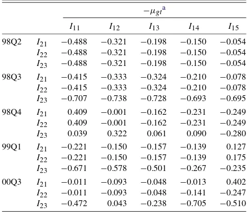
Table 7. The group index in the two random coefficient PCM
−µgta
NOTE: The reported indexes are based on the third column in Table2. Groups in the upper rows prefer a larger capacity of the level 2 cache and groups in the left columns prefer products of higher overall quality. The value of the outside option is identified with the assumption that on average△ξjtof the continuing products does not change.
a−µgt×100 gives a percentage change in price for groupgfromt−1 tot.
price decline. The other explanation is that the assumption that product quality linearly depends on product characteristics may not be appropriate to fully capture relationship between charac-teristics and product quality.
Table 7 reports the quality adjusted price index for con-sumer groups in the two random coefficient PCM for some selected periods. Consumers differ in their willingness to pay for quality improvement mainly measured by the processing speed (αi), and differ in their valuations on capacity of the
level 2 cache(βis). As a result, those who have the same value
ofαimay purchase different products because of different
val-ues ofβis.
In the table consumers are divided into 15 groups according to their values of αi andβis. Groups in the upper rows prefer
a larger capacity of the level 2 cache and groups in the left columns prefer products of higher overall quality. The table starts with the second quarter of 1998, one period before the introduction of Celeron processors, so the index in this period is the same across rows. In the following period the index in the third row is much lower than those in the first two rows, show-ing that consumers who do not care much about capacity of the level 2 cache become much better by Celeron processors.
In the fourth quarter of 1998 when Intel withdrew one Celeron processor (out of two) from the market, some groups in the third row became worse off. However, with a new line of Celeron processors introduced in the following quarter all groups in the third row experience a considerable decline in the index. This explains the difference between Table3and Table4 for the first quarter of 1999. The table also shows that a rela-tively modest decrease in the market index for the third quarter of 2000 is related to consumers who purchase Pentium proces-sors.
4. CONCLUSIONS
Using the pure characteristics demand model, I compute the quality adjusted price index for the CPU market. The index goes down by more than 25% when quality improves without a price increase. It goes down by less than 10% when no new product is introduced. It is comparable with the hedonic price index, but more sensitive to quality change.
I group consumers according to values of the random cients and compute the group index. In the one random coeffi-cient PCM consumers only differ in their willingness to pay for quality improvement. In the two random coefficient model con-sumers also differ in their willingness to pay for extra memory storage inside the processor. The group index shows how each group is affected by product entry and exit.
One caveat is that the index is based on a static demand model. This means that all consumers enter the market every period and buy at most one product. If they do not buy at all, it means that they decide not to own any product. This implies that the utility of products lasts for only one period. However, con-sumers purchase durable goods intermittently. Some concon-sumers already own products and decide whether to replace them with new ones.
A more proper price index should incorporate the durable good feature. If a consumer purchases a product for replace-ment, the index should be based on a utility difference between buying a new product and using her “old” product. A dynamic demand model that explicitly models a replacement decision is necessary to construct an index for durable goods.
ACKNOWLEDGMENTS
The author thanks Ana Aizcorbe, Ernst Berndt, Gary Cham-berlain, Iain Cockburn, Vivek Ghosal, Robert McClelland, Aviv Nevo, Ariel Pakes, Amil Petrin, Robert Porter, Manuel Trajten-berg, Jack Triplett, the Associate Editor, two anonymous ref-erees, and seminar participants at Cornell University, Purdue University, and the 2005 NBER summer institute for their sug-gestions and comments. All errors are mine.
[Received February 2008. Revised June 2008.]
REFERENCES
Berry, S. (1994), “Estimating Discrete-Choice Models of Product Differentia-tion,”Rand Journal of Economics, 25, 242–262. [191]
Berry, S., and Pakes, A. (2007), “The Pure Characteristic Demand Model,” In-ternational Economic Review, 48, 1193–1225. [190,191]
Berry, S., Levinsohn, J., and Pakes, A. (1995), “Automobile Prices in Market Equilibrium,”Econometrica, 63, 841–890. [190]
Bresnahan, F. (1987), “Competition and Collusion in the American Auto Indus-try: The 1995 Price War,” Journal of Industrial Economics, 35, 457–482. [191]
Griliches, Z. (ed.) (1971),Price Indexes and Quality Change: Studies in New Methods of Measurement, Cambridge, MA: The Harvard University Press. [190]
Nevo, A. (2003), “New Products, Quality Changes and Welfare Measures Com-puted From Estimated Demand Systems,”The Review of Economics and Statistics, 85 (2), 266–275. [190,194,195]
Pakes, A. (2003), “A Reconsideration of Hedonic Price Indices With an Application to PC’s,” American Economic Review, 93 (5), 1578–1596. [190,192,195,196]
Pakes, A., Berry, S., and Levinsohn, J. (1993), “Applications and Limitations of Some Recent Advances in Empirical Industrial Organization: Price Indexes and the Analysis of Environmental Change,”American Economic Review, Papers and Proceedings, 83, 240–246. [190,191]
Shaked, A., and Sutton, J. (1982), “Relaxing Price Competition Through Prod-uct Differentiation,”Review of Economic Studies, 49, 3–13. [191] Small, K. A., and Rosen, H. S. (1981), “Applied Welfare Analysis With Discrete
Choice Models,”Econometrica, 49, 105–130. [191]
Song, M. (2007), “Measuring Consumer Welfare in the CPU Market: An Ap-plication of the Pure Characteristics Demand Model,”RAND Journal of Economics, 38, 429–446. [191,193,195]
(2008), “Estimating the Pure Characteristics Demand Model: A Computational Note,” unpublished manuscript, University of Rochester, Rochester, NY. [193]
Trajtenberg, M. (1990),Economic Analysis of Product Innovation: The Case of CT Scanners, Cambridge, MA: The Harvard University Press. [190,191]