www.elsevier.com / locate / econbase
Imposing local concavity in the translog and generalized
Leontief cost functions
a b ,
*
David L. Ryan , Terence J. Wales
a
University of Alberta, Edmonton, Canada
b
University of British Columbia, Vancouver, Canada
Received 11 August 1999; accepted 21 October 1999
Abstract
We propose and illustrate a method for imposing concavity at a single point, which may result in concavity at many points, in the familiar Translog and Generalized Leontief cost functions, while at the same time maintaining flexibility of the forms. 2000 Elsevier Science S.A. All rights reserved.
Keywords: Cost functions; Local concavity; Negative semidefinite
JEL classification: C30
1. Introduction and general approach
We propose and illustrate, for the familiar Translog (TL) and Generalized Leontief (GL) cost functions, a simple method for imposing at a point the requirement that the cost function be concave in prices. As is well known, a necessary and sufficient condition for concavity is that the Hessian matrix of the cost function be negative semidefinite. To ensure that this condition is met at a reference point, we adapt a procedure that we developed and applied in the consumer demand context (Ryan and Wales, 1998).
Our interest in this topic stems partly from the results contained in a paper by Diewert and Wales (1987). They estimate the TL and GL cost functions using the data utilized by Berndt and Khaled (1979). The data contain information for the period 1947–1971 on output of U.S. manufacturing industries together with information on prices and quantities for four inputs: capital (K ), labour (L ), energy (E ) and materials (M ). They find that the TL violates concavity at 6 of the 25 sample points and the GL violates concavity at all of the sample points. Since imposing global concavity on either of
*Corresponding author. Tel.: 11-604-822-2876; fax:11-604-822-5915. E-mail address: [email protected] (T.J. Wales)
these forms destroys its flexibility, the authors dismiss these forms and are led instead to the development of more complex forms that allow concavity to be imposed globally, while at the same time maintaining flexibility.
In this paper we follow a different route and retain the TL and GL forms, but instead of imposing concavity globally, we impose it locally at a chosen reference point. Local imposition of concavity does not destroy the flexibility of the forms, and although it guarantees concavity at one point only, it may well be that a judicious choice of reference point leads to satisfaction of concavity at most or all
1
data points in the sample. This is what we find for several functional forms when applying the procedure in the consumer demand context (Ryan and Wales, 1998; 1999), and indeed this is what we find below for the TL and GL in the producer context. Thus at least for this data set, there is no need to abandon these familiar cost functions on account of their inability to satisfy the concavity in prices condition required by economic theory.
In brief, the procedure developed in Ryan and Wales (1998) in the consumer demand context to ensure negative semidefiniteness of the Slutsky matrix can be used in the producer context to ensure negative semidefiniteness of the Hessian matrix of the cost function. Thus, our procedure can be applied to any cost function provided it, together with its associated input demand system, contains a matrix of parameters A with the same number of independent elements as the Hessian matrix of the cost function H, and that at a chosen reference point, H can be written as H5A1 E, where E is a matrix with each element a function of some or all of the other parameters in the model, but not of A. Then using a general procedure proposed by Diewert and Wales (1987), negative semidefiniteness can be imposed on H as follows. First H is equated to a new matrix defined as 2DD9, where D is triangular, and second, A is replaced by 2DD9 2E in the demand equations. Estimation of the elements of D (rather than of A) and of the parameters in E guarantees that the Hessian matrix is
2
negative semidefinite at the reference point, as desired.
2. The translog and generalized Leontief cost functions
To permit comparison with the results of Diewert and Wales (1987), we specify the TL and GL cost functions to be the same as theirs. Thus, following these authors (p. 467), the TL cost function with n inputs is given by
In this paper we adhere to the definition of second-order flexibility given in Diewert (1974, p.113). A cost function is flexible if the level of cost and all of its first and second derivatives coincide with those of an arbitrary cost function that satisfies the linear homogeneity in prices property at any point in an admissible domain.
2
where p is a vector of n input prices, C( p, y, t) is cost, y is output, t is time and t* is the chosen
3
reference point; both t and t* take on values between 1 and 25. Necessary and sufficient conditions ensuring that C is linearly homogeneous in input prices are
O
ai51,O
aiy50,O
ait50, andO
aij50 for i51, . . . n (2)j
The corresponding TL share equations are given by
s ( p, y, t)i 5ai1
O
a ln pij j1a ln yiy 1a (tit 2t*) i51, . . . n (3)j
where s ( p, y, t) is the ith input’s share in cost. Without loss of generality we set all prices and outputi to one at the reference point t*, which gives si5a for all i at this point.i
Diewert and Wales (1987, p. 48) show that the Hessian of the TL cost function will be negative semidefinite, providing C( p, y, t).0, if and only if the matrix G given in (4) below is negative semidefinite. The ijth element of G, evaluated at t*, is defined as
gij5aij2ai ijd 1a ai j i, j51, . . . n (4)
with dij51 if i5j and 0 otherwise. Imposing curvature at the reference point is attained by setting
G5 2DD9 with D triangular, and solving for A as
aij5 2(DD9)ij1ai ijd 2a ai j i, j51, . . . n (5)
where (DD9) is the ijth element of DDij 9. The elements of A are replaced in the estimating equations with the right hand side of (5) thus guaranteeing that G, and hence H, is negative semidefinite. It is easy to see that reparameterizing according to (5) will not destroy the flexibility of the functional form because the n(n21) / 2 elements of D just replace the n(n21) / 2 elements of A in the estimation. Negative semidefiniteness of G guarantees concavity of the cost function at the reference point.
Following Diewert and Wales (1987, p.49) the GL cost function is given by
1 / 2 1 / 2 2
with bij5b for all i and j. Written in this form it is by no means evident that our procedure can beji
applied to the GL. However, a simple reparameterization of (6) allows us to impose local concavity. Without loss of generality we set ok bik50 for all i, and introduce n new parameters by adding soi
p d y to the right hand side of (6). This gives the following set of input demand equations to bei id
estimated, after normalizing by output
21 21 / 2 1 / 2 21 21 2
x yi 5
O
b pij i pj 1di1b yi 1b tit 1aity 1biy1git (7)j
3
where ok bik50 for i51, . . . n, and x is the quantity demanded of the ith input.i
The ijth element of the Hessian of the cost function for this system evaluated at the reference point, where all prices and output are unity, is then easily shown to be
h 5b / 2 i±j ij ij
(8)
5 2
O
b / 2ij 5b / 2ii i5jk±j
Thus, to impose concavity we set
bij5 2(DD9)ij i, j51 . . . n (9)
and replace the elements of B with those of D in the estimating equations. Negative semidefiniteness of B (and hence of H) guarantees concavity of the cost function at the reference point.
3. Empirical application
The TL system that we estimate consists of Eq. (1) and n21 of the equations in (3), while the GL consists of the n equations in (7). We add a vector of disturbances e to each system, and assume that the es are independent and that each has a multivariate normal distribution, with expectation zero and covariance matrix given by V, where V is constant over time. We maximize the likelihood function corresponding to each model under consideration.
In addition to estimating the models with concavity imposed locally using the methods described above, we also estimate versions in which concavity is not imposed, and we estimate versions in which concavity is imposed globally. In contrast to the imposition of curvature at a point, these global curvature restrictions destroy the flexibility of the cost functions. As discussed in Diewert and Wales (1987, p. 48) the TL will satisfy the concavity in prices property globally if, assuming positive shares, the matrix A is negative semidefinite. To impose this condition in the estimation (5) is replaced by
aij5 2(DD9)ij (59)
Unfortunately, imposing this condition may lead to seriously biased elasticity estimates.
A sufficient condition for global concavity of the GL cost function is that b $0 for all i±j. To ij
]2
impose this condition in the estimation, each b (i±j ) is replaced by k , and these k (i±j )
ij
œ
ij ijparameters are estimated in place of the b (i±j ). Unfortunately, imposing this condition destroys the ij
flexibility of the GL since it rules out complementarity between inputs.
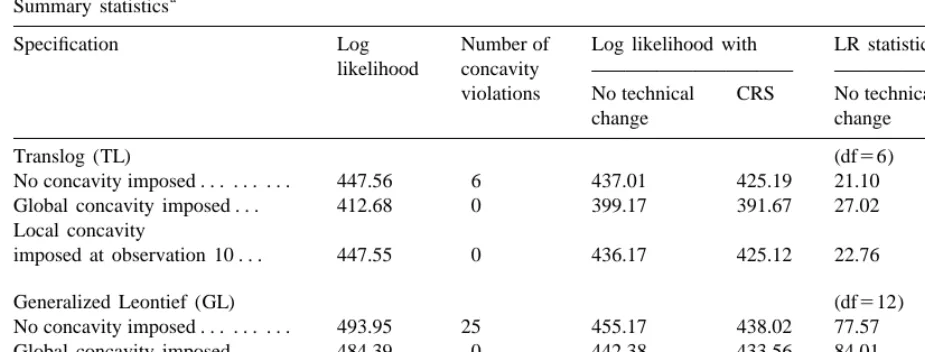
Table 1
a
Summary statistics
Specification Log Number of Log likelihood with LR statistics likelihood concavity
violations No technical CRS No technical CRS
change change
Translog (TL) (df56)
No concavity imposed . . . 447.56 6 437.01 425.19 21.10 44.74 Global concavity imposed . . . 412.68 0 399.17 391.67 27.02 42.01 Local concavity
imposed at observation 10 . . . 447.55 0 436.17 425.12 22.76 44.88
Generalized Leontief (GL) (df512)
No concavity imposed . . . 493.95 25 455.17 438.02 77.57 111.87 Global concavity imposed . . . 484.39 0 442.38 433.56 84.01 101.66 Local concavity
imposed at observation 1 . . . . 493.70 0 454.55 437.99 78.28 111.41
a
Notes: Sample size is 25. The restriction of no technical change requires 6 parameter restrictions in the TL: at50, ayt50, att50, and ait50, i51 . . . n21, and 12 parameter restrictions in the GL: bit5a 5 g 5i i 0, i51 . . . n. The CRS restriction involves 6 parameter restrictions in the TL: ay51, ayt50, ayy50, and aiy50, i51 . . . n21, and 12 parameter restrictions in the GL: bi5a 5 b 5i i 0, i51 . . . n.
originally violated at every sample point), imposition of curvature at the first observation results in the
4
curvature conditions being satisfied at all points.
As can be seen from the first column of Table 1, imposition of curvature at a point has very little effect on the value of the log likelihood function, although imposition of curvature globally causes a noticeable reduction in this value. The third and fourth columns of Table 1 show similar results for simpler formulations of the models in which there is no technical change or in which there are constant returns to scale (CRS). In addition, while the values of the Likelihood Ratio statistics for tests of each of these two hypotheses (columns 5 and 6) are similar for the models with no curvature imposed, or with curvature imposed locally, they are again quite different when curvature is imposed globally. In all cases the same conclusion (rejection) would be reached concerning these hypotheses, but the differences suggest that in contrast to imposing curvature at a point, the imposition of global curvature has different effects depending on the particular form of the model (with or without CRS or technical change) that is specified.
Price elasticities for the TL are obtained as:
´ij5a /sij i1sj2dij, (10) while for the GL they have the form:
1 / 2
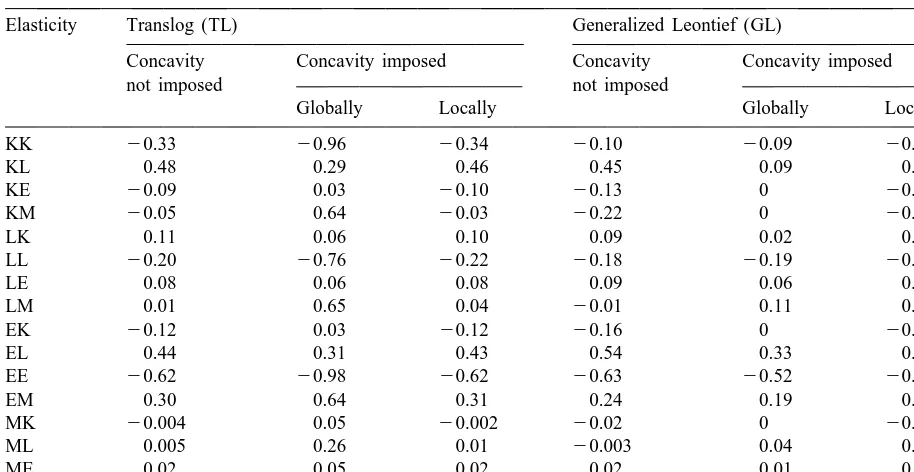
Table 2
Note: KL indicates the demand elasticity of capital (K) with respect to the price of labour (L). Other entries are defined analogously.
where dij51 if i5j, and 0 otherwise. Since these elasticities depend on data as well as parameters,
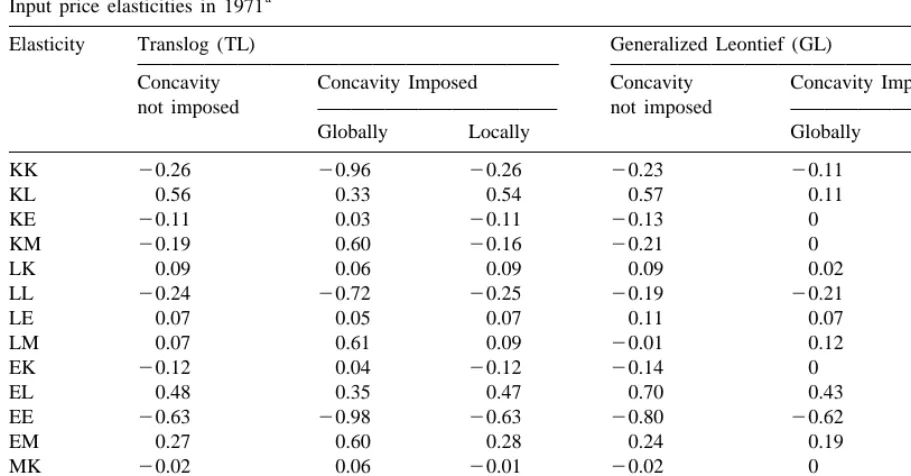
they differ over the sample period. To illustrate this variation, and any effect it has on the relationships between the elasticities for the various specifications, Table 2 contains these price elasticities for 1947 (the beginning of the sample period), while Table 3 contains the corresponding values for 1971 (the last year of the sample period). These elasticities are evaluated using the estimated shares (TL) and the estimated input–output ratios (GL) for the general models with no restrictions on returns to scale or technical change effects.
As can be seen from Tables 2 and 3, all input price elasticities are almost the same in the TL model where concavity is not imposed and in the TL model with concavity imposed locally. However, when concavity is imposed globally on the TL, the own-price elasticities become much larger in absolute value as do the elasticities of each input with respect to the price of materials (M). In addition, and in contrast to the other two TL specifications, all cross-price elasticities are positive in the TL model in which concavity is imposed globally, so that no pairs of inputs are complements. This latter result is not surprising in view of the related discussion in Diewert and Wales (1987, p. 48.)
Table 3
Note: KL indicates the demand elasticity of capital (K) with respect to the price of labour (L). Other entries are defined analogously.
model, b $0 (i±j ), ensures that ´ $0 (i±j ). It is interesting to note that in some cases this
ij ij
non-negativity restriction is binding to the point that certain bij50. As a result, the corresponding estimated cross-price elasticities are equal to zero throughout the sample.
In addition to input price elasticities, the effect of technological change on the inputs (≠ ln x /i ≠t)
and on total cost (≠ ln C /≠t) was determined for the various TL and GL specifications, although the
results are omitted here for brevity. While these technological change effects are very small throughout the sample period (despite the significance of the LR statistic in Table 1 that is used to test for technological change), an interesting finding is that they are virtually the same for all three TL specifications and for all three GL specifications. Thus, the effects of imposing concavity either locally or globally appear to be limited mainly to the price responses. This finding is also supported by the output elasticity of total cost (≠ln C /≠ln y), which is the same for all three TL models and all three GL models. However, the elasticities of each input with respect to output (≠ln x /i ≠ ln y) differ for some inputs for some observations when global concavity is imposed, although not when concavity is only imposed at a single observation.
4. Conclusion
locally does not guarantee its satisfaction at other points, we find that local imposition results in concavity being satisfied at all data points, for both forms. Thus, at least for the data set considered here, there is no need to resort to more complex functional forms that allow concavity to be imposed globally, while at the same time maintaining flexibility.
References
Berndt, E.R., Khaled, M.S., 1979. Parametric productivity measurement and choice among flexible functional forms. Journal of Political Economy 87, 1220–1245.
Diewert, W.E., 1974. Applications of duality theory. In: Intrilligator, M.D., Kendrick, D.A. (Eds.), Frontiers of Quantitative Economics, Vol.II, North Holland, Amsterdam, pp. 106–171.
Diewert, W.E., Wales, T.J., 1987. Flexible forms and global curvature conditions. Econometrica 55, 43–68.
Ryan, D.L., Wales, T.J., 1998. A simple method for imposing local curvature in some flexible consumer demand systems. Journal of Business and Economic Statistics 16, 331–338.