E-mail address:[email protected] (C.A. Sims)
Using a likelihood perspective to sharpen
econometric discourse: Three examples
Christopher A. Sims*
Department of Economics, Princeton University, Princeton, NJ 08544-1021, USA
Abstract
This paper discusses a number of areas of inference where dissatisfaction by applied workers with the prescriptions of econometric high theory is strong and where a likeli-hood approach diverges strongly from the mainstream approach in its practical prescrip-tions. Two of the applied areas are related and have in common that they involve nonstationarity: macroeconomic time-series modeling, and analysis of panel data in the presence of potential nonstationarity. The third area is nonparametric kernel regression methods. The conclusion is that in these areas a likelihood perspective leads to more useful, honest and objective reporting of results and characterization of uncertainty. It also leads to insights not as easily available from the usual perspective on infer-ence. ( 2000 Published by Elsevier Science S.A. All rights reserved.
JEL classixcation: C1
Keywords: Trend; Panel data; Kernel regression; Bayesian; Spline
1. Introduction
Many econometricians are committed, at least in principle, to the practice of restricting probability statements that emerge from inference to pre-sample probability statements }e.g. &If I did this analysis repeatedly with randomly drawn samples generated with a truebof 0, the chance that I would get abK as
big as this is 0.046'. Of course if we are to make use of the results of analysis of some particular data set, what we need is to be able to make a post-sample probability statement}e.g.,&Based on analysis of these data, the probability that
bis 0 or smaller is 0.046'. The latter kind of statement does not emerge as an
&objective' conclusion from analysis of data, however. If this is the kind of probability statement we aim at, the objective part of data analysis is the rule by which probability beliefs we held before seeing the data are transformed into new beliefs after seeing the data. But providing objective analysis of data that aims to aid people in revising their beliefs is quite possible, and is the legitimate aim of data analysis in scholarly and scienti"c reporting.
Pre- and post-sample probabilities are often closely related to each other, requiring the same, or nearly the same calculations. This is especially likely to be true when we have a large i.i.d. sample and a well-behaved model. This is one reason why the distinction between pre- and post-sample probability hardly ever enters the discussion of results in natural science papers. But in economics, we usually have so many models and parameters potentially available to explain a given data set that expecting &large' sample distribution theory to apply is unrealistic, unless we arti"cially restrict formal analysis to a small set of models with short lists of parameters. Econometric analysis generally does make such deliberate arti"cial restrictions. Applied econometricians and users of their analyses understand this as a practical matter and discount the formal probabil-ity statements emerging from econometric analyses accordingly. If the discount-ing is done well, the result need not be badly mistaken decisions, but the formal probability statements themselves can make econometricians look foolish or hypocritical. It would be better if econometricians were trained from the start to think formally about the boundaries between objective and subjective compo-nents of inference.
In this paper, we are not going to expand further on these broad philosophical points. Instead we are going to consider a series of examples in which a Bayesian approach is needed for clear thinking about inference and provides insights not easily available from standard approaches.
2. Possibly non-stationary time series
2.1. Why Bayesian and mainstream approaches diwer here
assumptions. Bayesian approaches that make the role of prior information explicit are therefore in con#ict with mainstream approaches that attempt to provide apparently objective rules for arriving at conclusions about low-fre-quency behavior.
Because mainstream approaches do not use probability to keep track of the role of non-sample information in determining conclusions about low frequency behavior, they can lead to unreasonable procedures or to unreasonable claims of precision in estimates or forecasts. When forecasting or analysis of behavior at low frequencies is the center of interest in a study, good research practice should insist on modeling so that the full range of a priori plausible low-frequency behavior is allowed for. Of course this is likely to lead to the conclusion that the data do not resolve all the important uncertainty, so that the model's implied probability bands will (accurately) appear wide and will be sensitive to vari-ations in auxiliary assumptions or (if explicitly Bayesian methods are used) to variations in the prior.
But mainstream approaches instead tend to lead to an attempt to "nd a model that is both simple and&acceptable' }not rejected by the data}and then to the making of probability statements conditional on the truth of that model. Parameters are estimated, and ones that appear&insigni"cant', at least if there are many of them, are set to zero. Models are evaluated, and the one that"ts best, or best balances "t against parsimony, is chosen. When applied to the problem of modeling low-frequency behavior, this way of proceeding is likely to lead to choice of some single representation of trend behavior, with only a few, relatively sharply estimated, free parameters. Yet because the data are weakly informative, there are likely to be other models of trend that"t nearly as well but imply very di!erent conclusions about out-of-sample low-frequency behavior.
The Bayesian remedy for this problem is easy to describe. It requires, for decision-making, exploring a range of possible models of low-frequency behav-ior and weighting together the results from them on the basis of their ability to
"t the data and their a priori plausibility. The exact weights of course depend on a prior distribution over the models, and in scienti"c reporting the aim will be to report conclusions in such a way that decision-makers with di!ering priors"nd the report useful. Where this is feasible, the ideal procedure is simply to report the likelihood across models as well as model parameters.
Good mainstream econometric practice can, by reporting all models tried that "t reasonably well, together with measures of their "t, and by retaining
&insigni"cant'parameters when they are important to substantive conclusions, give an accurate picture of the shape of the likelihood function.
information usable by people with varying priors, reporting a marginalized likelihood or marginalized posterior may not be helpful to people whose priors do not match the prior used in performing the integration (even if the likelihood itself has been integrated, implying a #at prior). Good reporting, then, will require doing a good job of choosing one or more priors that come close to the beliefs of many readers of the report. Reporting marginal posteriors under a range of priors can be thought of as describing the likelihood by reporting values of linear functionals of it rather than its values at points.
To this point we have simply applied to the context of modeling nonstation-ary data general principles concerning the di!erence between pre-sample and post-sample forms of inference. But there are some speci"c ways in which
&classical' approaches to inference either lead us astray or hide important problems from view.
2.2. Bias toward stationarity
In a classic paper in econometric theory, Hurwicz (1950) showed that least-squares estimates ofo in the model
y(t)"oy(t!1)#e(t)
e(t)DMy(s), s(tN&N(0,p2) (1) is biased toward zero. I think most people interpret this result to mean that, having seen in a given sample the least-squares estimate o(, we should tend to believe, because of the bias toward zero in this estimator, that probably the true value ofois greater thano(, i.e. that in thinking about the implications of the data for o we need to &correct' the biased estimator for its bias. As Sims and Uhlig (1991) showed, this is not true, unless one started, before seeing the data, with strong prior beliefs thatovalues near 1 are more likely than smallero values. The reason is that the bias is o!set by another e!ect: o( has smaller variance for largero's, a fact that by itself would lead us to conclude that, having seen the sample data, the trueois probably belowo(.
In this context, then, the presample probability approach gives us a mislead-ing conclusion. But though bias in this model does not have the implications one might expect, there is a serious problem with naive use of least-squares estimates in more complex autoregressive time series models, and classical asymptotic theory gives us misleading answers about it.
2.3. Implausible forecasting power in initial conditions
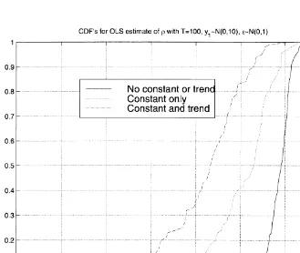
Fig. 1. CDFs of OLSo( wheno"1.
chance of explaining a lot of variation as emerging deterministically from initial conditions rises. When this happens, the results usually do not make sense. This situation is re#ected in the drastically increased (presample) bias when constant terms or constants with trends are added to the model, which is illustrated in the simple Monte Carlo results displayed in Fig. 1. But from a Bayesian perspective, the problem can be seen as the implicit use, in relying on OLS estimates, of a prior whose implications will in most applications be unreasonable.
The nature of the problem can be seen from analysis of the model that adds a constant term to (1),
y(t)"c#oy(t!1)#e(t). (2) This model can be reparameterized as
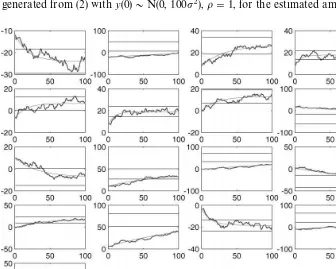
Fig. 2. Initial conditions Rogues'gallery. Note: Rougher lines are Monte Carlo data. Smoother curved lines are deterministic components. Horizontal lines are 95% probability bands around the unconditional mean.
variation into two components: a deterministic component, predictable from data up to time t"0, and an unpredictable component. The predictable component has the form
y6(t)"(y(0)!C)ot#C. (4) In the case where the true value ofcis zero and the true value ofois one, the OLS estimates (c(, o() of (c, o)"(0, 1) are consistent. ButCK"c(/(1!o() blows up as¹PR, becauseoP1 faster thancP0. This has the consequence that, even restricting ourselves to samples in which Do(D(1, the proportion of sample variance attributed by the estimated model to the predictable component does not converge to zero, but rather to a nontrivial (and fat-tailed) limiting distribu-tion. In other words, the ratio of the sum over the sample ofy6(t)2(as computed from (c(,o()) to the sum over the sample ofy(t)2does not converge to zero as
¹PR, but instead tends to wander randomly.
sample variance explained by the deterministic transienty6(0). Note that in all of these cases the initial value ofy(0) is outside the two-standard-error band about Cimplied by the OLS estimates. Clearly the OLS"t is&explaining'linear trend and initial curvature observed in these sample paths as predictable from initial conditions.
The sample size in each plot in Fig. 2 is 100, but the character of the plots is independent of sample size. This is a consequence of the scale invariance of Brownian motion. That is, it is well known that whether our sample of this discrete time random walk is of size 100 or 10,000, if we plot all the points on a graph of a given absolute width, and adjust the vertical scale to accommodate the observed range of variation in the data, the plot will look much the same, since its behavior will be to a close approximation that of a continuous time Brownian motion. Suppose we index the observations by their position s"t/¹ on (0, 1) when rescaled so the whole sample "ts in the unit interval. Suppose further that we scale the data so that the "nal y in the scaled datayH(¹)"y(¹)/J¹has variance 1. If we reparameterize (2) by settingd"
1/¹, c"cd, /"o!1/d, it becomes
yH(s#d)!yH(s)"d/(yH(s)!CJd)#Jde(t). (5) Eq. (5) is easily recognized as the standard discrete approximation, using small time intervald, to the continuous time (Ohrnstein}Uhlenbeck) stochastic di! er-ential equation
dyH(t)"/(yH(s)!CJd) dt#d=(t). (6) But in the limit as¹PR, yHis just a Brownian motion on (0, 1). We know that we cannot consistently estimate the drift parameters of a stochastic di! eren-tial equation from a"nite span of data. So we expect that for large¹we will have some limiting distribution for estimates of / and CJd. The limiting distribution for estimates of /implies a limiting distribution for estimates of (1!o)/¹"/, which is a standard result. But what interests us here is that the portion of the sample variation attributed to a deterministic component will also tend to a non-zero limiting distribution.
Of course the situation is quite di!erent, as ¹PR, when the data come from (2) withcO0 oroO1. WithcO0 ando"1, the data contain a linear trend component that dominates the variation. Our exercise of rescaling the data leads then, as¹PR, to data that looks just like a straight line, diagonally between corners of the graph. That is, in large samples the linear trend generated by cO0 dominates the variation. Not surprisingly then, the position of the trend line on the scaled graph is well estimated in large samples in this case. If
1Such cases lead to what they call&p-convergence'.
In applied work in economics, we do not know the values ofcoro, of course, but we do often expect there to be a real possibility ofcnear enough to 0 and
o near enough to 1 that the kind of behavior of OLS estimates displayed in Fig. 2, in which they attribute unrealistically large proportions of variation to deterministic components, is a concern.
It may be obvious why in practice this is&a concern', but to discuss the reasons formally we have to bring in prior beliefs and loss functions}consideration of what range of parameter values for the model are the center of interest in most economic applications, and what the consequences are of various kinds of error. Use of OLS estimates and the corresponding measures of uncertainty (standard errors,t-statistics, etc.) amounts to using a#at prior over (c, o). Such a prior is not#at over (C, o), but instead has density element D1!oDdCdo. That is, in (C,o) space it puts very low prior probability on the region whereoG1. There is therefore an argument for simply premultiplying the usual conditional likeli-hood function by 1/D1!oD. However, when as here di!erent versions of a&#at prior' make a di!erence to inference, they are really only useful as a danger signal. The justi"cation for using #at priors is either that they constitute a neutral reporting device or that, because often sample information dominates the prior, they may provide a good approximation to the posterior distribution for any reasonable prior. Here neither of these conditions is likely to hold. It would be a mistake to approach this problem by trying to re"ne the choice of
#at prior, seeking a somehow&correct'representation of ignorance.
There may be applications in which the#at prior on (c, o) is a reasonable choice. We may believe that initial conditions at the start of the sample are unrepresentative of the steady state behavior of the model. The start date of the model might for example be known to be the date of a major historical break, like the end of a war. Barro and Sala-I-Martin (1995, Chapter 11) display a number of cases where initial conditions are reasonably taken not to be drawn from the steady-state distribution of the process, so that a deterministic com-ponent is important.1
qualitatively di!erent from what has prevailed during the sample. The slope of the&trend line'will change, because the model implies that the data, over the time period¹#1,2,2¹, will be closer to its unconditional mean and thus less
strongly subject to mean-reversion pressures. Of course this could be the way the future data will actually behave, but believing this requires a"rm commit-ment to the restrictions on long-run behavior implicit in the parametric model. In accepting this prediction, we are agreeing to use a pattern in the observable data to predict a di!erent pattern of variation, never yet observed, in the future data.
There can be no universally applicable formula for proceeding in this situ-ation. One possibility, emphasized in an earlier paper of mine (Sims, 1989), is that we believe that a wide range of complicated mechanisms generating predictable low frequency variation are possible. What looks like a positive linear trend might just be a rising segment of a sine wave with wavelength exceeding the sample size, or of a second or third order polynomial whose higher-order terms start having strong e!ect only for tA¹. In this case the proper course is to recognize this range of uncertainty in the parameterization. The result will be a model in which, despite a good"t to low-frequency variation in the sample, uncertainty about long run forecasts will be estimated as high.
Another possibility, though, is that we believe we can use the existing sample to make long run forecasts, because we think it unlikely that there are such complicated components of variation at low frequencies. In this case, we believe that OLS estimates that look like most of those in Fig. 2 are a priori implausible, and we need to use estimation methods that re#ect this belief.
One way to accomplish this is to use priors favoring pure unit-root low-frequency behavior. An extreme version of this strategy is to work with di! er-enced data. A less extreme version uses a reference prior or dummy observations to push more gently in this direction. The well-known Minnesota prior for vector autoregressions (Litterman, 1983; Doan, 1992, Chapter 8) has this form, as does the prior suggested by Sims and Zha (1998) and the dummy observation approach in Sims (1993). A pure unit root generates forecasts that do not revert to a mean. It implies low-frequency behavior that will be similar in form within and outside the sample period. By pushing low-frequency variation toward pure unit root behavior, we tend to prevent it from showing oscillations of period close to¹.
2The classical distribution theory for the "xed-e!ect model describes the randomness in estimators as repeated samples are generated by drawingevectors with the values ofc
iheld "xed. For the random e!ects models it describes randomness in estimators as repeated samples are generated by drawing e vectors and c vectors. Though these two approaches usually are used to arrive at di!erent estimators, each in fact implies a di!erent distribution for any single estimator. That is, there is a random e!ects distribution theory for the"xed e!ects estimator and vice versa. There is no logical inconsistency in this situation, but if one makes the mistake of interpreting classical distribution theory as characterizing uncertainty about parameters given the data, the existence of two distributions for a single estimator of a single parameter appears paradoxical.
There are open research questions here, and few well-tested procedures known to work well in a wide variety of applications. More research is needed
} but on how to formulate reasonable reference priors for these models, not on how to construct asymptotic theory for nested sequences of hypothesis tests that seem to allow us to avoid modeling uncertainty about low-frequency components.
3. Possibly non-stationary dynamic panel data models
Here we consider models whose simplest form is
y
i(t)"ci#oyi(t!1)#ei(t), i"1,2,N, t"1,2,¹. (7)
Often in such models N is large relative to ¹. The common practice in time series inference of using as the likelihood the p.d.f. of the data conditional on initial conditions and on the constant term therefore runs into di$culty. Here there areNinitial conditionsy
i(0), andNconstant termsci, one of each
for each i. The amount of data does not grow relative to the number of free parameters, so they cannot be estimated consistently as NPR. This makes inference dependent, even in large samples, on the distribution of thec
i.
For a Bayesian approach, the fact that thec
ihave a distribution and cannot be
estimated consistently raises no special di$culties. There is no distinction in this approach between random c
i and ¶metric' ci. In approaches based on
pre-sample probability, by contrast, treating thec
ias random seems to require
a di!erent model (&random e!ects'), whose relation to the &"xed-e!ect' model can seem a philosophical puzzle.2
If the dynamic model is known to be stationary (DoD(1), with the initial conditions drawn randomly from the the unconditional distribution, then
3Ignoring observed data by constructing a likelihood for a subset of or a function of the data generally gives us a di!erent, less informative, likelihood function than we would get from all the data. But if the conditional distribution of the omitted data given the data retained does not depend on the parameters we are estimating, the likelihood for the reduced data set is the same as for the full data set.
which we can combine with the usual p.d.f. conditional on all the y
i(0)'s to
construct an unconditional p.d.f. for the sample. Maximum-likelihood estima-tion with this likelihood funcestima-tion will be consistent asNPR.
But if instead it is possible that DoD*1, the distribution of y
i(0) cannot be
determined automatically by the parameters of the dynamic model. Yet the selection rule or historical mechanism that produces whatever distribution of y
i(0) we actually face is critical to our inference. Once we have recognized the
importance of application-speci"c thinking about the distribution of initial conditions for the nonstationary case, we must also acknowledge that it should a!ect inference for any case where a root R of the dynamic model may be expected to have 1/(1!R) of the same order of magnitude as¹, which includes most economic applications with relatively short panels. When the dynamics of the model work so slowly that the e!ects of initial conditions do not die away within the sample period, there is generally good reason to doubt that the dynamic mechanism has been in place long enough, and uniformly enough acrossi, so that we can assumey
i(0),i"1,2,Nto be drawn randomly from the
implied stationary unconditional distribution fory
i(0).
It is well known that, because it makes the number of¶meters'increase with N, using the likelihood function conditional on all the initial conditions leads to bad results. This approach leads to MLEs that are OLS estimates of (7) as a stacked single equation containing the N#1 parameters Mc
i, i"
1,2,N, oN. These estimates are not consistent as NPR with ¹ "xed. An
alternative that is often suggested is to work with the di!erenced data. IfDoD)1, the distribution of*y
i(t), t"1,2,¹is the same acrossiand a function only of p2ando. Therefore maximum-likelihood estimation based on the distribution of the di!erenced data is consistent under these assumptions. Lancaster (1997) points out that this approach emerges from Bayesian analysis under an assump-tion thatDoD(1, in the limit as the prior on thec
ibecomes#at. (This Bayesian
justi"cation does not apply to the case where DoD"1, however, where the method is nonetheless consistent.)
Using the p.d.f. of the di!erenced data amounts to deliberately ignoring sample information, however, which will reduce the accuracy of our inference unless we are sure the information being ignored is unrelated to the parameters we are trying to estimate.3 If we are con"dent that (c
i, yi(0)) pairs are drawn
from a common distribution, independent acrossi and independent of the e i,
A simple approach, which one might want to modify in practice to re#ect application-speci"c prior information, is to postulate
(c
with the parameters of this distribution treated as unknown. This unconditional joint c.d.f. can then be combined with the conventional conditional c.d.f. for
My
i(t), t"1,2,¹, i"1,2,NNconditional on the initialyi(0)'s andci's, to
pro-duce a likelihood function. All the usual conditions to generate good asymptotic properties for maximum-likelihood estimates are met here asNPR.
Note that the setup in (9) is less restrictive than that in (8). The speci"cation in (8) gives a distribution for y
i(0) conditional on o,p2, and ci. If we use it to
generate a likelihood, we are implicitly assuming that none of these parameters a!ect the marginal distribution ofc
i. If we complete the speci"cation by
postu-latingc
These two restrictions reduce the number of free parameters by two, but do not contradict the more general speci"cation (9). The more general speci"cation gives consistent estimates asNPRregardless of the size ofDoD.
Of course where one is con"dent of the assumption of stationarity, it is better to use the restrictions embodied in (8), but in many economic applications it will be appealing to have a speci"cation that does not prejudge the question of stationarity.
No claim of great originality or wide usefulness is being made here for the speci"cation in (9). Similar ideas have been put forth before. The panel data context, because it is the home of the random e!ects speci"cation, has long been one where classically trained econometricians have had less inhibition about crossing the line between ¶meters' and &random disturbances'. Heckman (1981) proposes a very similar approach, and Keane and Wolpin (1997) a some-what similar approach, both in the context of more complicated models where implementation is not as straightforward.
Lancaster (1997) has put forward a di!erent Bayesian proposal. He looks for a way to reparameterize the model, rede"ning the individual e!ects so that a#at prior on them does not lead to inconsistent ML estimates. This leads him to di!erent priors when likelihood is the unconditional p.d.f. for the data imposing stationarity and when likelihood is conditional on initial conditions. In the latter case he"nds that this leads to an implicit prior on thec
parameterization that imposes a reasonable pattern of dependence between c
iand yi(0). His speci"cation does enforce an absence of dependence between
c
iandyi(0) wheno"1. While this will sometimes be reasonable, it is restrictive
and may sometimes distort conclusions. For example, if we are studying growth of incomey
i(t) in a sample of countriesiwhere the rich ones are rich because
they have long had, and still have, high growth rates, the c
i and yi(0) in the
sample will be positively correlated.
Applying the ideas in this section to more widely useful models in which right-hand side variables other than y
i(t!1) appear raises considerable
com-plications. A straightforward approach is to collect all variables appearing in the model into a single endogenous variable vectory
i, and then re-interpret (7) and
(9), making c
i a column and o a square matrix. Of course this converts what
started as a single-equation modeling problem into a multiple-equation prob-lem, but at least thinking about what such a complete system would look like is essential to any reasonable approach.
Another approach, closer to that suggested by Heckman (1981), preserves the single-equation framework under an assumption of strict exogeneity. We gener-alize (7) to
y
i(t)"oyi(t!1)#Xi(t)bi#ei(t), (12)
in which we assumeX
i(t) independent ofej(t) for alli,j, s,tin addition to the
usual assumption thate(t) is independent ofy
j(s) for alljOiwiths)tand for all
s(twithj"i. Now we need to consider possible dependence not just between a pair (y
i(0),ci), but among the vector MXi(s),bi,yi(0), s"1,2,¹N. It is still
possible here to follow basically the same strategy, though: postulate a joint normal unconditional distribution for this vector and combine it with the condi-tional distribution to form a likelihood function. One approach is to formulate the distribution as conditional on theXprocess, so that it takes the form
C
yi(0)
bi
DK
MXi(s), s"1,2,¹N&N(CXi, Rby), (13)whereXiis the¹-row matrix formed by stackingMX
i(t), t"1,2,¹N. Despite
the fact that the model speci"cation implies thaty
i(t) depends only onXi(s) for
s)t, we need to allow for dependence of the initialyon futureX's because they are related to the unobservableX
i(s) fors)0. IfNA¹, this should be a feasible,
albeit not easy, approach to estimation.
4. Kernel estimates for nonlinear regression
uncertainty more realistically than is possible in models with a small number of unknown parameters, and as a result they lead to implicitly or explicitly expanding the parameter space to the point where the degrees of freedom in the data and in the model are of similar orders of magnitude.
Kernel estimates of nonlinear regression functions do not emerge directly from any Bayesian approach. They do, though, emerge as close approximations to Bayesian methods under certain conditions. Those conditions, and the nature of the deviation between ordinary kernel methods and their Bayesian counter-parts, show limitations and pitfalls of kernel methods. The Bayesian methods are interesting in their own right. They allow a distribution theory that connects assumptions about small sample distributions to uncertainty about results in particular"nite samples, freeing the user from the arcane &order-Nq@p' kernel-method asymptotics whose implications in actual "nite samples often seem mysterious.
The model we are considering here is
y
i"c#f(xi)#ei, (14)
where thee
iare i.i.d. with variancep2, mean 0, independent of one another and
of all values ofx
j. We do not know the form off, but have a hope of estimating it
because we expect eventually to see a well dispersed set of x
i's and we believe
thatfsatis"es some smoothness assumptions. A Bayesian formalization of these ideas makes f a zero-mean stochastic process on x-space and c a random variable with a spread-out distribution. Though these ideas generalize, we consider here only the case of one-dimensional realx
i3R. Computations are
simple if we postulate joint normality for c, the f()) process and the e's. It is
natural to postulate thatc&N(0,l2), withl2large, and thatffollows a Gaus-sian zero-mean stationary process, with the covariances of f's at di!erent x's given by
cov(f(x
1), f(x2))"Rf(D(x1!x2)D) (15) for some autocovariance functionR
f. We can vary the degree of smoothness we
assume for f (including, for example, how many derivatives its sample paths have) by varying the form ofR
f.
The distribution of the valuey6(xH)"c#f(xH) of the regression functionc#f at some arbitrary pointxH, given observations of (y
i,xi), i"1,2,N, is then
4The e!ect of allowing for a large-prior-variancecin (14) is concentrated on making the integral of the kernel emerge as one.
where1is notation for a matrix"lled with one's. The distribution ofy6(xH) is then found by the usual application of projection formulas for Normal linear regres-sion, yielding
E[y6(xH)]"[y
1,2,yN]X~1W(xH), (18)
var[y6(xH)]"R
f(0)!W(xH)@X~1W(xH). (19)
A kernel estimate with kernelk, on the other hand, estimatesy6(xH) as
y(
Comparing (18) with (20) we see that the Bayesian estimate is exactly a kernel estimate only under restrictive special assumptions. Generally, the presence of a non-diagonal X matrix in (18) makes the way an observation (y
i, xi) is
weighted in estimating y6(xH) depend not only on its distance from xH (as in a kernel estimate), but also on how densely the region aroundx
i is populated
with observations. This makes sense, and re#ects how kernel methods are applied in practice. Often kernel estimates are truncated or otherwise modi"ed in sparsely populated regions of thex
ispace, with the aim of avoiding spurious #uctuations in the estimates.
There are a variety of classical approaches to adapting the kernel to local regions ofxspace (HaKrdle, 1990, Section 5.3). However, these methods empha-size mainly adapting bandwidth locally to the estimated shape off, whereas the Bayesian approach changes the shape of the implicit kernel as well as its bandwidth, and does so in response to data density, not the estimated shape off. A Bayesian method that adapted to local properties of f would emerge if cov(f(x
i), f(xj)) were itself modeled as a stochastic process.
There are conditions, though, under which the Bayesian estimates are well approximated as kernel estimates, even whenXis far from being diagonal. If the x
ivalues are equally spaced and sorted in ascending order, thenXis a Toeplitz
form (i.e. constant down diagonals), and to a good approximation, at least for inot near 1 orN, we can write (18) as
E[y6(xH)]"y(
k(xH) (21)
for
5In discrete time, the convolution of a function h with a function g is the new function
h*g(t)"+
sh(s)g(t!s).
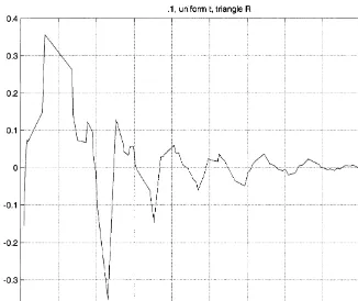
Fig. 3. Weighting function forxH"0.1. Nearestx
i: 0.0579, 0.0648, 0.1365, 0.1389.
convolution5 and the inverse is an inverse under convolution. Thus kernel estimates are justi"able as close to posterior means when the data are evenly dispersed and we are estimating y6(xH) for xH not near the boundary of the x-space. These formulas allow us to see how beliefs about signal-to-noise ratio (the relative size of R
f and p2) and about the smoothness of the f we are
estimating are connected to the choice of kernel shape. Note that forp2AR
f, we
havekGNp~2Rf!b, so that the kernel shape matchesRf. However it is not generally true that the kernel shape mimics that of theR
fthat characterizes our
prior beliefs about smoothness.
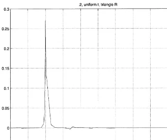
Fig. 4. Weighting function forxH"0.2. Nearestx
i: 6 between 0.1934 and 0.2028.
6The e!ects oflon the implicit kernels we plot below are essentially invisible. The e!ects would not be invisible for estimatedfvalues if the truechappened to be large.
kernel shape to the density of sampling in a given region}if only by making special adjustments at the boundaries of thex-space.
To illustrate these points we show how they apply to a simple example, in whichMx
i, i"1,2,100Nare a random sample from a uniform distribution on
(0, 1) and our model for f makes R
f(t)"max(1!DtD/0.12, 0). We assume p"0.17, making the observational error quite small relative to the variation in f, and set l"10.6In Fig. 3 we see weights that re#ect the fact thatxH"0.1 happens to fall in the biggest gap in thex
idata in this random sample. The gap is
apparent in the list of four adjacentx
i's given below the"gure. In contrast, Fig.
4 shows a case where the sample happens to contain manyx
i's extremely close to
xH. In this case there is no need to rely on distantx
i's. Simply averaging the ones
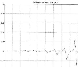
Fig. 5. Weighting function forxH"1. Nearestx
i: 0.9501, 0.9568, 0.9797, 0.9883.
7This follows from the fact thatW(xH) is by construction linear inxHover intervals containing no values ofx
ior ofxi$0.12.
The Bayesian approach to nonlinear regression described here is not likely to replace other approaches. IfR
fis chosen purely with an eye toward re#ecting
reasonable prior beliefs about the shape of f, the result can be burdensome computations when the sample size is large. TheXmatrix is of orderN]N, and if it has no special structure the computation ofX~1W(xH) is much more work than simply applying an arbitrarily chosen kernel function. The amount of work can be held down by, as in the example we have discussed, keeping the support ofR
fbounded, which makesXa constant matrix plus a matrix whose non-zero
elements are concentrated near the diagonal. It can be held down even further by special assumptions onR
f. Grace Wahba, in a sustained program of
theoret-ical and applied research (Wahba, 1990; Luo and Wahba, 1997), has developed
derivative (p*0) of thefprocess is a Brownian motion. In the example we have considered, our assumptions imply
f(x)"=(x)!=(x!0.12), (23) where= is a Brownian motion. Thus the special computational methods for smoothing splines do not apply to the example, though it can easily be veri"ed that the estimatedfin the example will be a continuous sequence of linear line segments, and thus a spline.7Generally, the result of the Bayesian method is a spline wheneverR
fis a spline, though it will not be a smoothing spline per se
for any choice of a stationary model forf.
5. Conclusion
The examples we have considered are all situations where realistic inference must confront the fact that the complexity of our ignorance is of at least the same order of magnitude as the information available in the data. Assumptions and beliefs from outside the data unavoidably shape our inferences in such situations. Formalizing the process by which these assumptions and beliefs enter inference is essential to allowing them to be discussed objectively in scienti"c discourse. In these examples, approaching inference from a likelihood or Bayesian perspective suggests some new interpretations or methods, but even where it only gives us new ways to think about standard methods such an approach will be likely to increase the objectivity and practical usefulness of our analysis by bringing our probability statements more into line with common sense.
Acknowledgements
The paper has bene"ted from comments by Tony Lancaster, Oliver Linton, and participants at the Wisconsin Principles of Econometrics Workshop.
References
Barro, R.J., Sala-I-Martin, X., 1995. Economic Growth. McGraw-Hill, New York. Doan, T.A., 1992. Rats User's Manual, Version 4. Estima, Evanston, IL 60 201.
HaKrdle, W., 1990. Applied Nonparametric Regression, Econometric Society Monographs, Vol. 19. Cambridge University Press, Cambridge, New York, New Rochelle, Melbourne, Sydney. Heckman, J.J., 1981. The incidental parameters problem and the problem of initial conditions in
Hurwicz, L., 1950. Least squares bias in time series. In: Koopmans, T.C. (Ed.), Statistical Inference in Dynamic Economic Models. Cowles Commission Monograph No. 10. Wiley, New York. Keane, M.P., Wolpin, K.I., 1997. Career decisions of young men. Journal of Political Economy 105,
473}522.
Lancaster, T., 1997. Orthogonal parameters and panel data. Working paper 97}32, Brown Univer-sity.
Litterman, R.B., 1983. A random walk, markov model for the distribution of time series. Journal of Business and Economic Statistics 1, 169}173.
Luo, Z., Wahba, G., 1997. Hybrid adaptive splines. Journal of the American Statistical Association 92, 107}116.
Sims, C.A., 1989. Modeling trends. Proceedings, American Statistical Association Annual Meetings. Sims, C.A., 1993. A 9 variable probabilistic macroeconomic forecasting model. In: Stock, J.H., Watson, M.W. (Eds.), Business cycles, Indicators, and Forecasting, Vol. 28. NBER Studies in Business Cycles, pp. 179}214.
Sims, C.A., Uhlig, H.D., 1991. Understanding unit rooters: A helicopter tour. Econometrica 59, 1591}1599.
Sims, C.A., Zha, T., 1998. Bayesian methods for dynamic multivariate models. International Economic Review.