Directory UMM :Data Elmu:jurnal:J-a:Journal of Econometrics:Vol101.Issue1.2001:

(1)

*Corresponding author. Tel.:#1-304-293-7871. E-mail address:vilasuso@be.wvu.edu (J. Vilasuso).

Causality tests and conditional

heteroskedasticity: Monte Carlo evidence

Jon Vilasuso

*

Department of Economics, College of Business and Economics, West Virginia University, P.O. Box 6025, Morgantown, WV 26506-6025, USA

Received 1 January 1997; received in revised form 1 March 2000; accepted 5 July 2000

Abstract

This paper investigates the reliability of causality tests based on least squares when conditional heteroskedasticity exists. Monte Carlo evidence documents considerable size distortion if the conditional variances are correlated. Inference based on a heteroskedas-ticity and autocorrelation consistent covariance matrix o!ers little improvement. This size distortion traces to an inability to discriminate between causality in mean and causality in variance. As a result, this paper endorses conducting causality tests based on an empirical speci"cation that explicitly models the conditional means and conditional variances. The relationship between money and prices serves as an illustrative

JEL classixcation: Classi"cation: C12; C15

Keywords: Simulation; ARCH

1. Introduction

Causality tests are routinely used to determine whether changes in one variable help explain movements in another variable. One popular approach is based on the work of Weiner (1956) and Granger (1969) and involves evaluating

(2)

1For comprehensive treatments of the de"nition of causality, see the papers included in the Journal of Econometrics Annals Issue (1988) entitled&Causalitya, edited by Dennis Aigner and Arnold Zellner.

2Andrews and Monahan (1992) and Cheung and Lai (1997) present Monte Carlo evidence that prewhitening is e!ective in reducing over-rejection. As a result, this paper uses prewhitened kernel estimators in the empirical work to follow.

a zero restriction in a vector autoregression (VAR).1Unfortunately, conclusions are often sensitive to alternative speci"cations of the time-series properties of the data. In the case of money and output, for example, researchers have shown that inference is sensitive to the lag speci"cation (Feige and Pearce, 1979), the method of time aggregation (Christiano and Eichenbaum, 1987), and the long-run properties of the data (Christiano and Ljungqvist, 1988; Stock and Watson, 1989). This paper examines the relationship between the time series properties of the data and statistical inference, focusing on whether conclusions based on causality tests using least-squares estimation are reliable if conditional hetero-skedasticity is present.

Results of Monte Carlo simulations suggest that conclusions drawn from least squares causality tests may lead to an erroneous claim that a statistically signi"cant causal relation exists. Misleading inference associated with least squares may be traced to two explanations. First, because the set of regressors in a VAR includes lagged-dependent variables, least-squares standard errors are not consistent and may not support correct statistical inference (Engle et al., 1985). Consequently, a logical way to proceed is to base inference on a hetero-skedasticity and autocorrelation consistent (HAC) covariance matrix. The use of a HAC covariance matrix, however, may not improve inference if there is &considerable'temporal dependence because kernel-based HAC covariance es-timators have test statistic values larger (in absolute terms) than that implied by the limiting distribution (Andrews and Monahan, 1992).2Hence, the null hy-pothesis of no causality is rejected too often.

A second explanation for the unsatisfactory performance of least-squares causality tests traces to a failure to adequately di!erentiate between causality in mean and causality in variance. This could prove particularly troublesome in practice, especially if interest is directed at asset pricing issues as Engle et al. (1990), Cheung and Ng (1996), and Lin (1997) document instances of volatility spillovers or causality in variance. Thus, if the poor performance of least-squares causality tests traces to an inability to di!erentiate between causality in mean and causality in variance, then causality tests are best based on a complete empirical speci"cation of the conditional means and conditional variances.

(3)

3Cheung and Ng (1996, p. 39) point out that causality in mean may a!ect tests for causality in variance. Causality in mean a!ects the structure of the disturbance terms, and in an autoregressive conditional heteroskedasticity model, the conditional variance is a linear function of the squared disturbances. On the other hand, causality in variance may also&have a possible, but smaller e!ect' on causality in mean tests because the conditional mean does not depend on the second moment (the ARCH-M model being an exception). In this paper, we numerically examine this latter e!ect.

4Note that a linear conditional mean model with ARCH disturbances can be described by a nonlinear speci"cation without ARCH, i.e. the bilinear model. In this paper, we assume that the conditional mean is linear and is correctly speci"ed in the simulations to follow.

problematic. However, if the conditional variances are correlated, there is considerable size distortion and a HAC covariance matrix o!ers only slight improvement. An apparent inability to di!erentiate between causality in mean and causality in variance is likely to present serious challenges in practice, and as a result, this paper recommends basing inference on an empirical model that explicitly models the conditional means and conditional variances.3The rela-tionship between money and prices serves as an illustrative example that statistical inference based on the least-squares framework and a fully speci"ed model di!ers widely.

2. Monte Carlo experiments

Monte Carlo experiments are used to assess the accuracy of statistical infer-ence based on least squares causality tests when conditional heteroskedasticity is present. Consider the mean-zero time series y_1,

t and y2,t for t"1, 2,2,¹ generated by a stationary VAR(1)

C

y zero serially uncorrelated disturbance terms with conditional covariance matrix

ij] and [aij] are matrices of coe$cients. The regression model speci"es a linear function for the conditional means where the disturbance terms are assumed to follow a"rst-order multivariate autoregressive conditional hetero-skedasticity (ARCH) model.4

The Monte Carlo experiments are designed such that [n

ij] is a lower triangular matrix which implies thaty

(4)

we set n₁₁"0.50,n₁₂"0,n₂₁"0.50, and n₂₂"0.25. Also, each element of [k

ij] is set equal to one. The data generating process forei,tis given bygi,tJhii,t whereg

i,tis i.i.d. N(0,1). The simulations consider a sample size of 100 and 500, using 5000 replications.

The experiments consider three di!erent parameterizations of [a

ij]. Model 1 serves as a benchmark and [a

ij] is set equal to the null matrix. In this case, the disturbance terms are homoskedastic, and least squares is consistent and e$cient.

The remaining models maintain that the disturbances exhibit condi-tional heteroskedasticity. The condicondi-tional covariance matrix for Model 2 is based on

Model 2 a"

C

0.2 0 0 0.9

D

.

Under Model 2, the conditional variances of the disturbance terms exhibit conditional heteroskedasticity but are unrelated. Because the set of regressors and the disturbances are correlated, least-squares standard errors are not consistent. The reliability of statistical inference is then potentially improved by constructing a HAC covariance matrix. The heteroskedasticity consistent estimator (HCE) developed by White (1980) is considered along with kernel-based HAC estimators popularized by Newey and West (1987) and Andrews (1991). We consider the Bartlett and Quadratic Spectral (QS) kernels where the bandwidth parameter is set according to the guide-lines presented by Newey and West (1994) where a VAR(1) is used to prewhiten prior to testing for causality in mean. A comparison of the results for Models 1 and 2 then examines whether least-squares causality tests are adversely a!ected by the inconsistency of the standard errors, and if so, whether a consistent estimator of the covariance matrix o!ers improve-ment.

Model 3 maintains that there is a causality in variance relation. The matrix [a

ij] is an upper triangular matrix which implies that the conditional variance of y

2,t causes the conditional variance ofy1,t, but given that [nij] is lower triangu-lar, y

2,t does not cause y1,t in mean. The conditional covariance matrix for Model 3 is based on

Model 3 a"

C

0.2 0.7 0 0.9

D

.

(5)

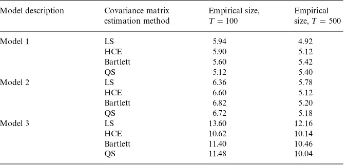
Table 1

Empirical size of nominal 5% causality in mean tests!

Model description Covariance matrix

Model 3 LS 13.60 12.16

HCE 10.62 10.14

Bartlett 11.40 10.46

QS 11.48 10.04

!Notes: The empirical size is based on 5000 replications of each model and¹denotes the sample size. Inference is based on least squares (LS), White's (1980) heteroskedasticity consistent estimator (HCE), and kernel-based HAC estimators of the covariance matrix. Kernels examined include the Bartlett and Quadratic Spectral (QS) kernels where the bandwidth parameter is set according to the guidelines o!ered by Newey and West (1994).

3. Simulation results

Table 1 summarizes the empirical test size associated with the null hypothesis thaty

2,tdoes not causey1,tin mean, which is true by construction. The nominal test size is 5%. Inference is based on the least-squares (LS) standard errors, White's (1980) heteroskedasticity consistent estimator, and a HAC covariance matrix using a Bartlett and Quadratic Spectral kernel computed under the least-squares framework.

For Model 1,e

1,t ande2,t are uncorrelated and are distributed i.i.d. N(0,1). Thus, least-squares is consistent and e$cient, and the empirical test size should not di!er from the nominal test size. As shown in Table 1, this is the case as the empirical test size is approximately equal to the nominal test size.

The empirical test size based on the least-squares standard errors for Model 2 is approximately equal to the nominal test size for¹"_{500. This suggests that if} [a

(6)

choice of kernel is of secondary importance compared to the choice of the bandwidth parameter. Comparing results for Models 1 and 2 suggests that the inconsistency of the least-squares standard errors is not particularly harmful if the conditional variances are unrelated, although a HAC estimator of the covariance matrix does improve inference for larger samples.

Tests results based on the least-squares standard errors for Model 3, however, are markedly di!erent. There is considerable size distortion, and constructing a HAC covariance matrix o!ers only slight improvement. This "nding likely traces to an inability to discriminate between causality in mean and causality in variance. That is, when there is causality in variance, inference based on least squares and a HAC covariance matrix is apt to erroneously claim that there is causality in mean.

4. The money}price relation

This section explores the relationship between money and prices in an e!ort to gauge the performance of least-squares causality tests in practice. Friedman and Schwartz (1963) espouse the Monetarist claim that money causes prices in mean via the quantity equation. However, it is certainly plausible that causality runs from prices to money. If the monetary authorities condition policy at least in part on past in#ation, then lagged in#ation helps explain movements in intermediate or indicator variables which include money (see, e.g. Fuhrer and Moore, 1995).

The causal structure linking money and prices is examined for the period 1964:I}1997:III. Seasonally adjusted, quarterly data for money and prices were obtained from the St. Louis Federal Reserve data"les. M1 serves as a measure of money and the CPI represents the price level. As noted by Hoover (1991), M1 is an appropriate measure of money because M1 served as the primary monetary aggregate used by the monetary authorities for much of the sample period.

(7)

5We also tabulated a critical value of the SupF test based on bootstrap simulations because the testing procedure developed by Bai and Perron (1997) is asymptotic, and in some cases dividing the full sample results in small subsamples. In any event, the asymptotic and bootstrap values both suggest a signi"cant trend break at the 5% level.

6Consistent with Stock and Watson (1989), we"nd no evidence that prices and money are cointegrated.

7Ball and Cecchetti (1990), among others, also detect conditional heteroskedasticity for in#ation. 8Monte Carlo results reported by Cheung and Ng (1996) indicate that the two-stage maximum likelihood test possesses good empirical size and power properties.

test developed by Bai and Perron (1997) and"nd a statistically signi"cant break in trend money growth that occurs in 1991 (not shown).5In the empirical work to follow, we work with log-di!erenced prices and detrended log-di!erenced M1, both with and without a trend break.6

Causality in mean test results are summarized in Table 2. Causality tests constructed under the least squares framework evaluate a zero restriction in a estimated VAR which includes four lagged terms as suggested by Akaike's Information Criterion. Panel A examines whether money causes prices, and Panel B focuses on whether prices cause money. Beginning in Panel A, statistical inference based on least squares standard errors and a HAC covariance matrix support the claim that money causes prices at the 5% signi"cance level. Turning to Panel B, there is little evidence that prices cause money. Thus, causality test results constructed under the least-squares framework support the Monetarist claim that money causes prices.

There is, however, evidence of conditional heteroskedasticity. The Ljung and Box (1978) portmanteau test for up to sixth-order serial correlation applied to the squared disturbances is signi"cant at the 1% level in the price equation for both descriptions of money (not shown).7Engle's (1982) Lagrange multiplier test (not shown) rejects the homoskedastic null hypothesis at the 5% signi"cance level for the squared disturbances from the price and money equations, regard-less of whether a trend break in money growth is included. Consequently, the least-squares framework may not support accurate statistical inference, parti-cularly if the time-varying conditional variances are correlated.

(8)

Table 2

Money}price causality in mean tests, 1964:I}1997:IV!

Measure of money Covariance matrix estimation

method

Detrended M1 Detrended M1 with trend break

A.p-values for the hypothesis that all coe$cients on lagged money in the price equation are zero. Least-squares framework

LS 0.05 0.05

HCE 0.04 0.02

Bartlett 0.02 0.02

QS 0.02 0.02

Maximum likelihood

Multivariate 0.35 0.17

Univariate 0.44 0.22

B.p-values for the hypothesis that all coe$cients on lagged prices in the money equation are zero. Least-squares framework

LS 0.14 0.19

HCE 0.16 0.17

Bartlett 0.24 0.23

QS 0.18 0.20

Maximum likelihood

!Notes: Kernel-based HAC estimators of the covariance matrix use a VAR(1) to prewhiten. Multivariate (quasi) maximum likelihood causality in mean tests are based on a multi-variate ARCH(1) speci"cation, and the unimulti-variate (quasi) maximum likelihood causality in mean tests are based on an AR(4) with ARCH(1) residuals. Maximum likelihoodp-values are based on the Bollerslev and Wooldridge (1992) standard errors

9The ARCH(1) speci"cation appears to adequately "t the data. Likelihood ratio tests reject homogeneity at the 1% signi"cance level for each speci"cation, and Ljung}Box tests applied to the squared standardized residuals do not indicate statistically signi"cant serial correlation.

framework, results shown in Table 2 indicate that causality tests based on maximum likelihood techniques o!er evidence that prices cause money, consis-tent with the reaction function literature and "ndings reported by Hoover (1991).9

(9)

Table 3

Money}price causality in variance tests, 1964:I}1997:IV!

Measure of money

Estimation method Detrended M1 Detrended M1 with trend break A.p-values for the hypothesis that prices do not cause money in variance.

Maximum likelihood

B.p-values for the hypothesis that money does not cause prices in variance Maximum likelihood

!Notes: See notes to Table 2.

10See Bollerslev et al. (1992) for a discussion of this literature.

conditional variance of money causes the conditional variance of prices. Thus, the least-squares conclusion that money causes prices in mean likely traces to an inability to di!erentiate between causality in mean and causality in variance.

5. Conclusion

This paper demonstrates that if conditional heteroskedasticity is ignored, least squares causality tests exhibit considerable size distortion if the conditional variances are correlated. Moreover, inference based on a HAC covariance matrix constructed under the least squares framework o!ers only slight im-provement. The poor performance of least squares causality tests traces to an inability to di!erentiate between causality in mean and causality in variance if the regression disturbances are incorrectly assumed to be homoskedastic. Con-sequently, this paper recommends that causality tests be based on an empirical speci"cation that models both the conditional means and the conditional variances.

(10)

likelihood function proves daunting if a large number of time series is included or if a long lag structure is used to specify the conditional means. In these cases, the univariate maximum likelihood causality tests proposed by Cheung and Ng (1996) represent an attractive alternative.

References

Andrews, D.W.K., 1991. Heteroskedasticity and autocorrelation consistent covariance matrix es-timation. Econometrica 59, 817}858.

Andrews, D.W.K., Monahan, J.C., 1992. An improved heteroskedasticity and autocorrelation consistent covariance matrix estimator. Econometrica 60, 953}966.

Bai, J., Perron, P., 1997. Estimating and testing linear models with multiple structural changes. Econometrica 66, 47}78.

Ball, L., Cecchetti, S.G., 1990. In#ation and uncertainty at short and long horizons. Brookings Papers on Economic Activity 1, 215}254.

Bollerslev, T., Chou, R.Y., Kroner, K.F., 1992. ARCH modeling in"nance. Journal of Econometrics 52, 5}59.

Bollerslev, T., Wooldridge, J.M., 1992. Quasi-maximum likelihood estimation and inference in dynamic models with time varying covariances. Econometric Reviews 11, 143}172.

Cheung, Y.W., Lai, K.S., 1997. Bandwidth selection, prewhitening, and the power of the Phillips-Perron test. Econometric Theory 13, 679}691.

Cheung, Y.W., Ng, L.K., 1996. A causality-in-variance test and its application to"nancial market prices. Journal of Econometrics 72, 33}48.

Christiano, L.J., Eichenbaum, M., 1987. Temporal aggregation and structural inference in macro-economics. In: Brunner, K., Meltzer, A. (Eds.), Carnegie-Rochester Conference Series on Public Policy. North-Holland, New York, pp. 63}130.

Christiano, L.J., Ljungqvist, M., 1988. Money does cause output in the bivariate money-output relation. Journal of Monetary Economics 22, 217}235.

Dickey, D.A., Pantula, S.G., 1987. Determining the order of di!erencing in autoregressive processes. Journal of Business & Economic Statistics 5, 455}461.

Engle, R.F., 1982. Autoregressive conditional heteroskedasticity with estimates of the variance of U.K. in#ation. Econometrica 50, 987}1008.

Engle, R.F., Hendry, D.F., Trumble, C., 1985. Small-sample properties of ARCH estimators and tests. Canadian Journal of Economics 17, 66}93.

Engle, R.F., Ito, T., Lin, W., 1990. Meteor showers or heat waves? Heteroskedastic intra-daily volatility in the foreign exchange market. Econometrica 58, 525}542.

Feige, E.L., Pearce, D.K., 1979. The causal relationship between money and income: Some caveats for time series analysis. Review of Economics and Statistics 61, 21}33.

Friedman, M., Schwartz, A.J., 1963. A Monetary History of the United States. Princeton University Press, Princeton.

Fuhrer, J.C., Moore, G.R., 1995. Monetary policy trade-o!s and the correlation between nominal interest rates and real output. American Economic Review 85, 219}239.

Granger, C.W.J., 1969. Investigating causal relations by econometric models and cross spectral methods. Econometrica 37, 424}438.

Hoover, K.D., 1991. The causal direction between money and prices: An alternative approach. Journal of Monetary Economics 27, 381}423.

(11)

Ljung, G.M., Box, G.E.P., 1978. On a measure of lack of"t in time-series models. Biometrika 65, 297}303.

Newey, W.K., West, K.D., 1987. A simple, positive semi-de"nite, heteroskedasticity and autocorrela-tion consistent covariance matrix. Econometrica 55, 703}708.

Newey, W.K., West, K.D., 1994. Automatic lag selection in covariance matrix estimation. Review of Economic Studies 61, 631}653.

Stock, J.H., Watson, M.W., 1989. Interpreting the evidence on money-income causality. Journal of Econometrics 40, 161}181.

Weiner, N., 1956. The theory of prediction. In: Beckenback, F.F. (Ed.), Modern Mathematics for the Engineer. McGraw-Hill, New York, pp. 165}190.