isprsannals II 3 W5 187 2015

(1)

ASSESSMENT OF THE THEMATIC ACCURACY OF LAND COVER MAPS

J. Höhle

Dept. of Planning, Aalborg University, Skibbrogade 3, DK-9000 Aalborg, Denmark – jh@plan.aau.dk

Commission II, WG II/4

KEY WORDS: Land Cover Map, Urban, Classification, Machine Learning, Assessment, Accuracy, Confidence Interval

ABSTRACT:

Several land cover maps are generated from aerial imagery and assessed by different approaches. The test site is an urban area in Europe for which six classes (‘building’, ‘hedge and bush’, ‘grass’, ‘road and parking lot’, ‘tree’, ‘wall and car port’) had to be derived. Two classification methods were applied (‘Decision Tree’ and ‘Support Vector Machine’) using only two attributes (height above ground and normalized difference vegetation index) which both are derived from the images. The assessment of the thematic accuracy applied a stratified design and was based on accuracy measures such as user’s and producer’s accuracy, and kappa coefficient. In addition, confidence intervals were computed for several accuracy measures. The achieved accuracies and confidence intervals are thoroughly analysed and recommendations are derived from the gained experiences. Reliable reference values are obtained using stereovision, false-colour image pairs, and positioning to the checkpoints with 3D coordinates. The influence of the training areas on the results is studied. Cross validation has been tested with a few reference points in order to derive approximate accuracy measures. The two classification methods perform equally for five classes. Trees are classified with a much better accuracy and a smaller confidence interval by means of the decision tree method. Buildings are classified by both methods with an accuracy of 99% (95% CI: 95%-100%) using independent 3D checkpoints. The average width of the confidence interval of six classes was 14%

of the user’s accuracy.

1. INTRODUCTION

Land cover maps can automatically be derived from satellite or aerial imagery. There exist many different methods to classify the objects in the landscape based on imagery. One approach is a supervised classification where one uses a selection of reference units to train the applied classifier in order to achieve a high thematic accuracy. The assessment of the thematic accuracy uses samples and estimates the accuracy of the whole map. In a stratified random sampling scheme, samples are taken for each class and the thematic accuracy is estimated for each class. Important is the reliability of the derived accuracy measures. They should, therefore, be supplemented by confidence intervals. There exist different methods to derive confidence intervals. The derivation may use the maximum likelihood or bootstrapping method. For the maximum likelihood method, the formulae can be found in (Card, 1982). In the present contribution, the bootstrap method is applied. It may be used for samples with normal or non-normal distribution of the errors. In order to test the usefulness of the approach, a few land cover maps will be produced and assessed. Two different classification methods are applied: The Decision Tree (DT) and the Support Vector Machine (SVM). The theoretical background of the two methods is given in previous publications, e.g. (Breiman et al., 1984) and (Vapnik, 1998). The basic idea in SVM method is to find an optimal hyperplane which separates two classes with the maximum distance between the closest training units (xi). The mathematical

formulation is a cost function

where w is the normal to the hyperplane, ξi are variables which

account for the non-separability of data, and the constant C represents a regularization parameter that allows to control the penalty assigned to errors. The cost function is minimized using e.g. a Gaussian Kernel function K(xi, x)=exp(-γ||xi-x||2) where γ

is a parameter inversely proportional to the width of the Kernel. A detailed description of the SVM method is given in (Melgani and Bruzzone, 2004) from where the above formula is taken. The DT method uses an algorithm in order to split the training data so that an optimal homogeneity of a class within a subset is achieved. The classification and regression tree (CART) algorithm, e.g., uses the ‘Gini impurity’ as a measure for how often a randomly chosen training unit would be incorrectly labelled. This can be expressed in the formula

where fi isthe fraction of units labelled with class i. (Wikipedia,

2015a). Both methods have been employed for the generation of land cover maps using various remotely sensed data. In this contribution, the data are from an aerial camera with four spectral bands. The images overlap and are of high resolution and geometric quality. Such data enable new approaches for the derivation of land cover maps. Height data can be derived and used as an effective feature in the classification. Aerial imagery of three bands have been used together with lidar data in (Trinder and Salah, 2011). Reference data were obtained by digitizing polygons of the four classes (‘building’, ‘road’, ‘tree’,

‘ground’) in the orthoimage. The use of the SVM method revealed an overall accuracy of 96.8%. Experiences with DT classification are published, e.g. in (Hansen et al., 1996), (Friedl and Brodley, 1997). (Gerke and Xiao, 2014) used airborne laser



_ 

 m

i i

G f f

I

1 2

) 2 ( 1

) (

) 1 ( ||

|| 2 1 ) , (

1 2



_  

 N

i i

C w

w 

(2)

scanning point clouds and image data of four bands to derive land cover maps with four classes by the Random Forest method. A test example of a residential area revealed thematic accuracies of 96.2% (‘building’), 96.7 (‘tree’), 98.9% (‘sealed

ground’), and 88.0% (‘vegetated ground’). The reference values were determined by an operator and partly used to train the RTrees classifier. Tests with aerial imagery of four bands and DT classification were also carried out in (Höhle and Höhle, 2013) in order to generate land cover maps of urban areas with four and six classes. Height data were derived from the images. Good results could also be obtained with a DT where the splitting rules were manually selected based on a-priori contextual information. The refinement of the automatically derived land cover maps by means of image processing methods has successfully been implemented in (Höhle, 2014). The main emphasis in this contribution is the methodology of assessment of the thematic accuracy. Also for this task, 3D data can be used with advantage. The structure of this paper is the following: Section 2 discusses the assessment of the thematic accuracy in general. The applied tools are presented in Section 3. Section 4 contains practical tests with the derivation of a land cover map of an urban area. The obtained land cover maps are assessed by different methods in Section 5. Discussion and conclusion in Section 6 and 7 complete the paper.

2. THE ASSESSMENT OF THE THEMATIC ACCURACY IN GENERAL

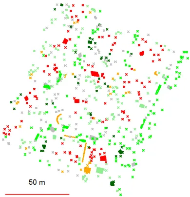
The assessment of the thematic accuracy of each class requires checkpoints (aka reference points). Their position is randomly selected and a class value has to be determined at these positions with a high accuracy and reliability. Such points (or cells) are the reference data. Their number has influence on the reliability of the estimated thematic accuracy and, hence, the sample size becomes an important issue of the accuracy assessment. Various authors developed methods and formulae for this task, e.g. (Tortora, 1978), Congalton and Green, 2009), (Höhle and Höhle, 2013). In the last reference the calculations are carried out by means of functions, available as open source. The checkpoints should be completely independent from the training areas. Figure 1 depicts training areas and checkpoints used in the generation and assessment of a land cover map.

Figure 1. Training areas and randomly selected checkpoints (crosses). The colours represent different classes.

Image pairs and orthoimages, both in false colour, are sources for the reference (check-) points by which the assessment of the thematic accuracy is carried out. In the first case the checkpoints can be in 3D, which allows stereo-viewing of the checkpoint. As it is described so far, various methods are available for the assessment of the thematic accuracy. Some tests regarding the selection of checkpoints will also be carried out. Based on the gained experience in these tests, recommendations will be given.

2.1 Error matrix

The derived class for a cell is compared with the reference value. A matrix representation will give an overview on the agreement between the reference and the calculated class. The diagonal of this so-called error matrix (aka confusion matrix) contains the number of scores and the positions outside the diagonal are the errors (disagreements). The totals of the rows and columns supplement the error matrix, which is also used for the calculation of the accuracy measures. Weights are not

applied in this ‘raw’ error matrix.

2.2 Accuracy measures

The measures which characterize the thematic accuracy of a land cover map are the user’s and the producer’s accuracy, the overall accuracy and the kappa value. The formulae for these measures are published in (Congalton & Green, 2009). Other accuracy measures are commission and omission errors which can be derived by (100% - user’s accuracy) and (100% -

producer’s accuracy) respectively. If the goal is to estimate the accuracy for each class, a stratified simple random (STSI) sampling is applied. The sample size per class (nc) has to be

calculated assuming a worst-case user accuracy for each class and a desired width of the confidence interval. The sample of each class is found by simple random sampling without replacement. The total number of units (points/cells) in the sample is then n = nc∙k, where k is the number of classes.

Classes might be over- or under-sampled compared to their distribution in the produced land cover map. Therefore, weights are applied for each class of the sample. They are calculated using

) 3 (



 

i i i

n n N N w

where N is the total number of units in the map, Ni is the total

number of units of class ”i" in the map, n is the total number of units in the sample, ni+ is the number of units of class “i" in the

sample. Thereby, the stratified sampling design is taken into account. This ‘survey weighting’ is preferred because the sizes of classes and samples usually differ. At wi=1 all evaluated units

are treated equally. Approximations for the accuracy measures can be obtained by cross validation (cv). In this approach the set of reference data is split into cells for training of a DT and cells for validation. There exist several variants, we apply “Leave one out cross-validation”. The class label of one cell is predicted by a classifier, which is derived from the (n-1) cells. The reference value is not used for the classification of this cell. The procedure is repeated n times resulting in n different classifiers. From the assigned class values an error matrix can be formed and approximate accuracy measures may be derived. Cross validation is usually used in order to test the applied model (selection of variables or parameters) or to compare different methods of classification (Wikipedia, 2015b). Because the ISPRS Annals of the Photogrammetry, Remote Sensing and Spatial Information Sciences, Volume II-3/W5, 2015

(3)

training data are not completely independent from the test data accurate and reliable accuracy measures are not obtainable by cross validation.

2.3 Confidence intervals

Each accuracy measure should also include a confidence interval (CI), which is a measure of the reliability of the accuracy measure. The distance between the lower and upper limit is the width of the CI. The calculated CI covers the true, but unknown, value of the accuracy measure with a confidence level of 95% if sampling is repeated many times. In 5% of all samples, the CI will not contain the true value of the accuracy measure. If the confidence level and the sample size are selected and kept fixed, the width of the CI depends only on the variability of the observations in the sample. It is of interest to the user that the width of the CI is a small value. The calculated accuracy measures are then more reliable. The calculation of the CIs should therefore be part of any assessment of the thematic accuracy of land cover maps.

3. TOOLS

There are several tools available for the generation of land cover maps and for the assessment of their accuracy. It has been one of the goals in this investigation to solve the tasks by open source software and by own programming. The R language and environment is the preferred tool (R Development Core Team, 2013).

3.1 R-packages

The open source programming language and environment ‘R’ provides several packages and functions, which ease the calculation of the sample size, the thematic accuracy and the confidence interval. The package ‘survey’ includes functions for the analysis of complex survey samples (Lumley, 2015). Functions of the package ‘binomSamSize’ compute confidence intervals and the necessary sample sizes (Höhle, 2015). The package ‘binom’ has functions for binomial confidence intervals (Dorai-Raj, 2015). Applied packages for the classification methods and for generation of the land cover maps are ‘rpart’ (decision trees from training data), ‘ipred’ (prediction of class values by means of the derived DT), and

‘kernlab’ (SVM classification). These R-packages are described in detail in (Therneau et al., 2015), (Peters et al., 2015), and (Karatzoglou et al., 2004).

3.2 Other tools

The professional programs ‘Match-T’, ‘DTMaster’, and

‘OrthoMaster’ of the Trimble/Inpho GmbH are useful for the

tasks in pre-processing. ‘Match-T’ generates gridded Digital

Surface Models (DSMs) from overlapping images. ‘DTMaster’

has functions for 3D data collection, filtering and editing of DSMs. 3D viewing of image pairs and automatic positioning to checkpoints are also valuable features of this software package.

‘OrthoMaster’ generates orthoimages.

4. PRACTICAL TESTS

The practical test is carried out with land cover maps of an urban area produced by means of different methods. We

describe first the area and the data at disposal, the steps in the classification for two different methods follow.

4.1 Test site

The test site is an urban area in Europe, which contains vegetated and non-vegetated objects. Buildings, car ports, walls, roads, and parking lots belong to the first category; the second category comprises the areas with grass, hedges, bushes and trees. A few swimming pools and paths are also part of the test site. The area covers about 1.4 ha.

4.2 Data

The test site has been imaged by a medium-format aerial camera (Leica RCD30). The images have four bands (red, green, blue, and near infra-red). The radiometric resolution of each band is 8 bit or 256 intensity values. The size of the pixel on the ground is 5 cm x 5 cm only. The high resolution images were taken in the morning of a sunny summer day which resulted in long shadows. Accurate orientation data (camera calibration data, spatial position of the perspective centre in the reference system (UTM/WGS84/Ellipsoidal Heights), and attitude of the camera axis) were provided.

4.3 Pre-processing

Pairs of colour images are first processed to a Digital Surface Model (DSM). The point cloud is generated by means of matching corresponding image points and by interpolating a regular grid of elevations thereafter. The spacing between the grid points was selected with 0.25 m. Each cell of 0.25 m x 0.25 m is considered as an object, which is supplemented with a number of attributes. For example, the height above ground (dZ), the normalized difference vegetation index (NDVI) or the intensity values of the four spectral bands (spectral signatures) may be chosen. These attributes have to be derived. The dZ- value is the difference between the DSM and the Digital Terrain Model (DTM). The DTM is processed by filtering of the DSM. Some editing of the DSM and the DTM may be required. The DTM is also a prerequisite for the generation of an orthoimage. Orthoimages are produced as false-colour composites where the vegetation is clearly seen.

4.4 Classification

The tasks for the classification are the selection of classes and attributes, the extraction of training points, and the selection of parameters at the applied classification methods in the practical tests. Two methods, ‘Decision Tree’ and ‘Support Vector

Machine’, will be used and compared.

The selection of classes and of the class attributes is an important step in the generation of a land cover maps. Starting point is the type of landscape, but the requirements of the map users and the characteristics of the available data may also decide on the number and the type of classes. In the applied high-resolution imagery small objects can automatically be detected. The achievable accuracy of the selected classes may differ considerably. The overall accuracy of a land cover map will depend on the selection of classes. In the practical example six classes are chosen and the accuracy of each class shall be determined. The selected classes are ‘building’, ‘hedge & bush’,

‘grass’, ‘road’, ‘tree’, and ‘wall & car port’. In order to separate the chosen classes from each other, a number of attributes have to be selected. The normalized difference vegetation index and ISPRS Annals of the Photogrammetry, Remote Sensing and Spatial Information Sciences, Volume II-3/W5, 2015

(4)

the height above ground are effective attributes for the chosen classes. Good results for the thematic accuracy require a training of the classifiers. This is accomplished by means of points, where the class is known. The extraction of training points is carried out on top of the false-colour orthoimage. The corner points of the chosen training areas are digitized and the spatial coordinates (E, N, Z) of each DSM-cell within the polygon are extracted and supplemented by the associated attributes. Altogether, 17449 DSM cells were collected which is about 2% of the total number of cells in the test area. In average, 2900 cells of one class will be used to train the classifier.

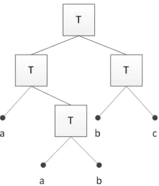
The DT-classification method determines thresholds for attributes which split the training data into two branches by means of an algorithm. The procedure is repeated several times until all training data are separated into the selected classes. The result is a tree with branches and leaves (cf. Figure 2), which gives the classification the name. This so-called ‘recursive

partitioning’ is easy to implement, but an effective performance of the DT requires reliable training data and attributes. The accuracy of the training points may be determined in advance (cf. section 5.3). Big deviations from 100% will indicate noise in the training areas, which then may deteriorate the accuracy of the land cover map. By means of the derived decision tree all cells of the DSM are assigned with one of the six classes. The cells can then be plotted with a colour for each class. The produced land cover map is georeferenced and contains 907339 cells.

Figure 2. Principle of decision tree classification (T=test using thresholds of attributes; a, b, c=classes). Modified after (Friedl and Brodley, 1997)

The SVM method is often applied for hyperspectral imagery where hundreds of spectral bands have to be handled. This method separates two classes by means of a hyperplane. A few points with attributes of each class are required to train the classifier. The calculated support vectors are weights, which select training points defining the optimal separating hyperplane. In the multi-class classification altogether M=k∙ (k-1)/2 classifications have to be carried out. The appropriate class is found by a voting scheme (cf. Figure 3). In our example with

six classes, M=6∙5/2=15 classifications thus have to be carried

out. The attributes of the points are usually the spectral signatures, i.e. the intensity values of each band. This approach leads to a long feature vector for multispectral imagery. It is good practice to reduce the number of features beforehand.

Figure 3. Solving multi-class problems with binary SVMs (x=feature vector, class=classification result). Modified after (Melgani and Bruzzone, 2004).

In this test, the normalized difference vegetation index is used which can separate the vegetated objects from non-vegetated objects efficiently. In addition, the height above ground is used for discriminating objects on the ground from objects above ground. This attribute is also known as ’nDSM’ which stands for normalized Digital Surface Model. In order to generate a land cover map with six classes, we use the function “ksvm” of the R-package ‘kernlab’. For this multi-class classification 15 binary classifiers are trained and 15 class values are predicted for each cell of the DSM. The maximum number is then the predicted class value. When several classes reach the maximum

number, the prior probability values decide on the “winning class”. The fractions of the areas, which the single classes cover,

are appropriate estimates for the prior probability values. The training of the classifier depends very much on the quality of the training areas. Noise in these data may exist but its influence is reduced by a regularization parameter (C). The selection of

‘C’ is empirical and a set of values is used. The best result is selected for the derivation of the land cover map. The calculation of the separating hyperplane uses a kernel function.

As kernel function, we select the “Gaussian radial basis function” (“rbfdot”) where the kernel parameter (γ) is set to

“automatic”. A value for the inverse kernel width is derived automatically. Figure 4 depicts the resulting land cover map.

Figure 4. Result of the classification by means of the SVM- method. (Red=’building’, light green=’grass’, dark green=’tree’, green=’hedge&bush’, grey=’road&parking lot’,

orange=’wall&car port’)

It is georeferenced. The selected regularization parameter is C=1. The used prior values were selected with 0.21 (‘building’), 0.18 (‘hedge&bush’), 0.25 (‘grass’), 0.19 (‘road&parking lot’), ISPRS Annals of the Photogrammetry, Remote Sensing and Spatial Information Sciences, Volume II-3/W5, 2015

(5)

0.04 (‘tree’), 0.13 (‘wall&car port’). 22% of the total area is covered with class ‘building’, 13% with class ‘hedge&bush’, 23% with class ‘grass’, 17% with class ‘road&parking lot’, 8% with class ‘tree’, and 17% with class ‘wall&car port’.

5. ASSESSMENT OF THE THEMATIC ACCURACY AND ITS RESULTS

The assessment of the derived land cover maps requires reference data (checkpoints). The number of checkpoints is calculated with 91 per class assuming a worst-case user accuracy of about 60% for each class and a desired width of the 95% confidence interval of ±10%. Details of the calculation are given in (Höhle and Höhle, 2013). At six classes, the total number of checkpoints amounts to 91∙6=546 checkpoints. The position of the checkpoints is randomly for each class. From all points of the derived land cover map, which were assigned with a certain class, a sample of 91 points is extracted. This is a stratified random sampling scheme. A reference value has to be determined at these random positions (cf. crosses in Figure 1). This so-called ‘true’ value can be found in the stereo pair or in the orthoimage. Such points are independent from the training areas. In the following, the results of the assessment are separated according to the data source and the type of checkpoints (2D or 3D). The type of classification will also be distinguished. The results of the assessments will be presented by means of the error matrix, the user’s and producer’s accuracy for each class, the overall accuracy, and the kappa coefficient. Each of the mentioned accuracy measures will be supplemented by a 95% confidence interval (95% CI). Weighting according equation (3) is applied due to the inequality of the class areas.

5.1 Assessment of the DT classification by means of independent 3D checkpoints

The reference data are found by means of observations in the original false-colour images. The 3D viewing is enabled by displaying the images in red and cyan and the use of glasses (filters) with the complementary colours (anaglyph method). The checkpoints must have spatial coordinates (E,N,Z) and can then be positioned and seen in 3D. The analyst observes the reference value and completes the “accuracy sample” with the reference value and the weight (cf. Table 1).

id nr E N Z c r w

546 922 537152.7 5228892.0 492.8 b b 1

Table 1. Excerpt of the “accuracy sample” in the assessment

with independent 3D checkpoints (id=index, nr=number, E=Easting, N=Northing, Z=elevation, c=classification, r=reference, w=weight).

By means of the “accuracy sample” with 546 observations an error matrix is computed (cf. Table 2). It reveals that the class

‘wall and car port’ cannot be determined well enough. Especially, the discrimination of this class from the class ‘road and parking lot’ is poor. The calculated user’s and producer’s accuracy for each class can be taken from Tables 3 and 4. The derived values are supplemented with confidence intervals. The overall accuracy is calculated with 79% (95% CI: 76%-82%), the kappa coefficient with 0.74 (95% CI: 0.70-0.77). ‘Survey

weighting’ has been applied in both measures. The average of the producer’s accuracy is 80% and of the users accuracy 73%.

The omission and commission errors are in average 20% and 27% respectively.

reference

class b h g r t w

row

Σ

b 90 0 1 0 0 0 91

h 0 71 17 1 1 1 91

g 3 8 74 5 0 1 91

r 5 2 0 82 1 1 91

t 10 4 6 0 71 0 91

w 8 8 8 43 0 24 91

col Σ 116 93 106 131 73 27 546 Table 2. Error matrix of the land cover map derived by a DT (b=’building’, h=’hedge&bush’, g=’grass’, r=’road&parking lot’, t=’tree’, w=’wall&car port’). Taken from (Höhle, 2014).

class accuracy 95% CI

building 99% 95%-100%

hedge&bush 78% 69%-86%

grass 81% 72%-89%

road&parking lot 90% 83%-95%

tree 78% 69%-86%

wall&car port 26% 18%-36%

Table 3. User’s accuracy of the derived land cover map by DT- classification

building 86% 80%-91%

grass 80% 74%-85%

tree 89% 71%-98%

Table 4. Producer’s accuracy of the derived land cover map by DT- classification

5.2 Assessment of the SVM classification by means of independent 3D checkpoints

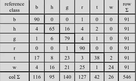
The numerical results of the assessment are contained in Tables 5-7. The error matrix of the SVM classification reveals rather

big commission errors in the classes ‘tree’ and ‘wall and car port’. The overall accuracy is 75% (95% CI: 73-78%) and the kappa coefficient is 0.70 (95% CI: 0.66-0.73). Both values are

‘survey weighted’, i.e. weights are applied according to the proportions of the class areas. The accuracies for the classes

‘tree’ (42%) and ‘wall and car port’ (26%) are poor and differ

considerably from the other four classes. reference

class b h g r t w

row

Σ

b 90 0 0 1 0 0 91

h 4 65 16 4 2 0 91

g 1 6 79 4 1 0 91

r 0 0 1 90 0 0 91

t 17 8 23 3 38 2 91

w 4 16 21 25 1 24 91

col Σ 116 95 140 127 42 26 546 Table 5. Error matrix of the SVM-classification (abbreviations for classes are explained in the caption of Table 2)

(6)

building 99% 95%-100%

grass 87% 79%-93%

tree 42% 32%-52%

Table 6. User’s accuracy of the individual classes (SVM- classification)

grass 70% 65%-75%

tree 82% 64%-94%

Table 7. Producer’s accuracy of the individual classes (SVM- classification)

5.3 Assessment by means of 2D checkpoints from training areas

Such checkpoints are usually close to each other and very likely correlated. Therefore, they are not independent checkpoints and the derived accuracy measures may be wrong. However, for comparison of different methods or for checking the noise in the training data, the use of such checkpoints may also be useful. We will carry out an experiment and select either a small sample or use all the cells of the training areas in order to assess the accuracy of the classification. The cells of the small sample are again randomly extracted from each class (strata). These points are not aligned. The class value of these points is known, the checkpoints serve as reference points. Table 8 contains the

user’s accuracy with CI’s, which are derived from a few randomly selected checkpoints (-cells) of the training areas. The

achieved user’s accuracy is close to 100%, the width of the CI’s

is ±4% in average. The overall accuracy is 96% (95% CI: 94-97%) and the kappa coefficient is 0.95 (95% CI: 0.93-0.97). Weights were again applied.

building 100% 100%-100%

grass 91% 84%-95%

tree 99% 92%-100%

Table 8. User’s accuracy with CIs derived from 6∙91=546 randomly selected cells of the training areas (SVM-classification)

The size of the sample can be extended and all cells of the training areas may be used. This is an aligned sampling. The

derived user’s accuracy with all training data are then compared with the assessment of the map accuracy using the sample of independent checkpoints extracted from the land cover map by stratified random sampling (cf. Table 9 and Section 5.1). The derived accuracies are all higher when cells from the training areas are used. This is expected. Of interest is how much the accuracies differ from 100%. Big deviations from 100% indicate noise in the training area of that class, which will influences the thematic accuracy of that class. For example, the

accuracy of the class ‘wall and car port’ of the derived land

cover map (using the DT-method) is far off (26%). Also, the assessment by means of all training data of this class revealed a reduced accuracy (73%).

class nc accuracy nc accuracy

building 4204 100% 91 99%

hedge&bush 3308 99% 91 78%

grass 2680 93% 91 81%

road&parking lot 3152 100% 91 90%

tree 1829 92% 91 78%

wall&car port 2276 73% 91 26% Table 9. User’s accuracy determined either by 17449 training points or by 546 independent points (DT-classification)

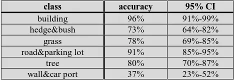
5.4 Assessment by means of 3D checkpoints using cross validation

In the test with cross validation, the 546 3D checkpoints are used for the derivation of the DT (in order to produce the land cover map) and partly for the assessment of its thematic accuracy (using cv). Table 10 depicts the derived error matrix and Table 11 the user’s accuracy.

reference/

class b h g r t w

row

Σ

b 96 0 1 1 1 1 100

h 0 69 19 1 1 4 94

g 3 9 78 7 0 3 100

r 1 3 2 112 1 4 123

t 8 4 6 0 70 0 88

w 8 8 0 10 0 15 41

col Σ 116 93 106 131 73 27 546 Table 10. Error matrix at cross validation (DT classification)

The error matrix reveals that the class ‘wall and car port’ (w) cannot be distinguished very well from the other classes. The

user’s accuracy will therefore be poor for this class.

grass 78% 69%-85%

tree 80% 70%-87%

Table 11. User’s accuracy with CIs derived by cross validation (DT classification)

The class ‘wall and car port’ is indeed poorly determined and the CI is rather big. The commission errors are in average 24%.

6. DISCUSSION

Two different methods have been used to classify an urban area. The assessment of the thematic accuracy uses stratified sampling with a sample size of nc=91 points in both

assessments. Checkpoints are determined randomly for each class of the final land cover map. They are independent from the training areas. The overall accuracy obtained by DT ISPRS Annals of the Photogrammetry, Remote Sensing and Spatial Information Sciences, Volume II-3/W5, 2015

(7)

classification (79%) is slightly higher than the one obtained by the SVM classification (75%). The results of both methods

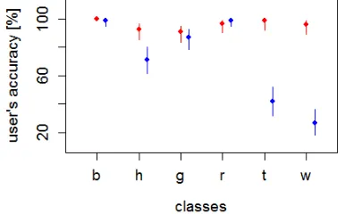
regarding user’s and producer’s accuracy are depicted in Figures 5 and 6.

Figure 5. User’s accuracy with confidence intervals for two methods of classification (Red=DT, blue=SVM, nc=91).

Abbreviations of classes are explained in Table 2.

Figure 6. Producer’s accuracy with confidence intervals for two

methods of classification (Red=DT, blue=SVM, nc=91).

Abbreviations of classes are explained in Table 2.

The user’s accuracy is for both methods about the same in five classes. For the class ‘tree’, however, the DT method produced a higher accuracy (78% vs. 42%). The confidence intervals are about the same for five classes. Again, class ‘tree’ reveals a bigger difference (ΔCI=3%). The CIs are in average 14% with a standard deviation of ±5% (DT method) and 14% and ±7% (SVM method). Regarding the producer’s accuracy (cf. Figure 6) the results of the individual classes are in average more balanced and of higher accuracy. The average CIs are with 18% ±10% (DT method) and 15%±8% (SVM method) higher than at the DT method. The size of CIs is between 14% and 18%, which is relative big, which supports the argument that there is no need to quote the thematic accuracy with decimals. In all tests, the required limit of ±10% for CIs is complied with. The sample size of nc=91 has, therefore, been properly selected. In

the SVM method the selection of the regularization parameter (C) has had influence on the results. Tests with a set of C-values {0.1, 1, 60, 100} revealed slight differences in the training errors. A change in the separation of classes could not be observed.

The number of cells used for training of the DT will be discussed in the following. We restrict to the user accuracy because it characterizes the derived land cover map. When checkpoints from the training data are used, the obtained accuracy differs. Figure 7 displays the user’s accuracy for the SVM classification. This is derived either from 546 points of the training data by means of mono observations of the ‘truth’ in the orthoimage (named ‘Training’) or from 546 points which

are sampled from the derived land cover map and use of stereo

observation of the ‘truth’ (named ‘Independent’). The used sample size is 91 points (cells) per class in both assessments.

Figure 7. User’s accuracy with confidence intervals for two types of checkpoints, sample size: nc=91, classification method:

SVM. (Red=Training, Blue=Independent). Abbreviations for classes are explained in Table 2.

The diagram in Figure 7 reveals for the assessment by means of a few (randomly selected) points of the training areas high accuracies (>90%) for all classes. The accuracies derived from independent checkpoints are considerably lower; for the classes

‘hedge and bushes’ (Δ=12%), ‘tree’ (Δ=42%) and ‘wall and car

port’(Δ=70%). These big differences confirm the general rule that the assessment of the thematic accuracy requires independent checkpoints.

Figure 8 depicts the comparison between the user’s accuracy derived by independent checkpoints and by cross validation (cf. Tables 3 and 11). The decision tree (which produced the land cover map) has been derived either from the training areas with 17449 cells (extracted from an orthoimage) or from the 546 3D points only.

Figure 8. User’s accuracy at DT classification (red=independent checkpoints , green=cross validation, nc=91)

The differences between the two approaches are small. A higher accuracy by the cross validation is obtained for three classes only (‘road and parking lot’, ‘tree’, ‘wall and car port’). The

other three classes (‘building’, ‘hedge and bush’, ‘grass’) reveal even a lower accuracy. The averaged widths of the CIs are 2.2% bigger in the cv approach.

7. CONCLUSION

The assessment by stratified sampling requires the derivation of the land cover map at first. Afterwards the samples can be taken for each class randomly. The determination of the reference

(‘truth’) is best done with georeferenced original images and by means of 3D viewing. The checkpoints have then to be with three coordinates (E,N,Z). The other choice for a source of reference data are orthoimages. When they are based on DTMs, positional errors at objects above ground will exist. ISPRS Annals of the Photogrammetry, Remote Sensing and Spatial Information Sciences, Volume II-3/W5, 2015

(8)

Observations of the reference in 2D are less reliable. The use of false-colour composites is of advantage because the vegetated areas are clearly visible. Aerial imagery of known exterior orientation and the application of stereo viewing is a reliable procedure for the assessment of the thematic accuracy. Training data are used for deriving the classifiers. Errors (noise) in the training data will influence the accuracy of the land cover map. The accuracy of the training units should therefore be assessed in order to produce accurate land cover maps. By means of a portion of training points the selection of attributes and parameters (e.g. C-values in SVM) in the applied model should be validated. For the assessment of the thematic accuracy we prefer 3D points derived from georeferenced false-colour images. We apply also weights for each class of the sample in order to compensate for over- or under-sampling. All derived accuracy measures are supplemented by 95% confidence intervals in order to check their reliability. The use of large-scale multispectral imagery of high geometric and radiometric quality is also a characteristic of this contribution. Accurate DSMs can then be derived and the DSM cells can be supplemented by nDSM and NDVI values. These effective attributes enable simple classification methods such as DT and SVM. Positional errors in the map and in reference data are avoided. All of these characteristics give the applied methodology in the generation and assessment of land cover maps advantages to other approaches.

ACKNOWLEDGMENTS

The author thanks Leica Geosystems for providing image data for these investigation. Michael Höhle, University of Stockholm, is thanked for support in programming and advices in statistical matters. The comments of the anonymous reviewers are appreciated.

REFERENCES

Breiman, L., Friedman, J., Stone, C.J., Olshen, R.A., 1984. Classification and regression trees. CRC press.

Card, D. H., 1982. Using known map category marginal frequencies to improve estimates of thematic map accuracy. Photogrammetric Engineering and Remote Sensing, 48 (3), pp. 431-439.

Congalton, R. G., Green, K., 2009. Assessing the accuracy of remotely sensed data. CRC Press, 183 p.

Dorai-Raj, S., 2015. “binom: Binomial confidence intervals for

several parameterizations”, R package version 1.1-1, 2015, http://cran.r-project.org/web/packages/binom/binom.pdf (11 March 2015).

Friedl, M.A., Brodley, C.E., 1997. Decision Tree Classification of Land Cover from Remotely Sensed Data. Remote Sensing of Environment 61, pp. 399-409.

Gerke, M. and Xiao, J, 2014. Fusion of airborne laserscanning point clouds for supervised and unsupervised scene classification. ISPRS Journal of Photogrammetry and Remote Sensing 87, pp. 78-92.

Hansen, M., Dubayah, R., DeFries, R., 1996. Classification trees: an alternative to traditional land cover classifiers. International Journal of Remote Sensing 17 (5), pp. 1075-1081.

Höhle, J., Höhle, M., 2013. Generation and assessment of urban land cover maps using high-resolution multispectral aerial cameras. International Journal on Advances in Software, vol 6, no 3 & 4, pp. 272-282. http://www.iariajournals.org/software/ (6 June 2015).

Höhle, J., 2014. Generation of 2D land cover maps for urban areas using decision tree classification. ISPRS Annals of the Photogrammetry, Remote Sensing and Spatial Infor mation Sciences, vol. II-7, pp. 15-21.

Höhle, M., 2015. Package ‘binomSamSize: Confidence

intervals and sample size determination for a binomial proportion under simple random sampling and pooled

sampling”, version 0.1-3, 18 p. http://cran.r-project.org/web/packages/binomSamSize/binomSamSize.pdf (15 March 2015).

Karatzoglou, A., Smola, A., Hornik, K., Zeileis, A. , 2004. Kernlab - An S4 package for kernel methods in R. Journal of Statistical Software, 11(9), pp. 1-20.

Lumley, T. , 2015. R package "survey". http://cran.r-project.org/web/packages/survey/survey.pdf (11 March 2015).

Melgani, F., Bruzzone, L., 2004. Classification of hyperspectral remote sensing images with support vector machines, IEEE Transactions on Geoscience and Remote Sensing, 42 (8), pp. 1778-1790.

Peters, A., Hothorn, T., Brian D. Ripley, B. D., Therneau, T., Atkinson, B., 2015. “ipred: Improved predictors”, R-package

version 0.9-4,

http://cran.r-project.org/web/packages/ipred/ipred.pdf (11 March 2015).

R Development Core Team, 2013. R: A language and environment for statistical computing, http://www.r-project.org (13 March 2015).

Therneau, T., Atkinson, B., Ripley, B. D., 2015. “rpart: Recursive partitioning”, R package, version 4.1-9. http://cran.r-project.org/web/packages/rpart/rpart.pdf (11 March 2015).

Tortora, R., 1978. A note on sample size estimation for multinomial populations. The American Statistician, 32(3), pp. 100-102.

Trinder, J. C., M. Salah, M., 2011. Support Vector Machines: Optimization and validation for land cover mapping using aerial images and lidar data. Proceedings of the 34th International Symposium on Remote Sensing of Environment, Sydney/Australia, 10-15 April 2011, 4 p.

http://www.isprs.org/proceedings/2011/ISRSE-34/211104015Final00895.pdf (8 March 2015).

Vapnik, V. N., 1998. Statistical Learning Theory. Wiley, New York.

Wikipedia, 2015a. Decision tree learning, http://en.wikipedia.org/Decision _tree_learning (14 June 2015)

Wikipedia, 2015b. Cross-validation (statistics), http://en.wikipedia.org/wiki/Cross-validation_(statistics). (30 April 2015).