DISOCCLUSION OF 3D LIDAR POINT CLOUDS USING RANGE IMAGES
P. Biasuttia, b, J-F. Aujola, M. Br´edifc, A. Bugeaub
aUniversit´e de Bordeaux, IMB, CNRS UMR 5251, INP, 33400 Talence, France. b
Universit´e de Bordeaux, LaBRI, CNRS UMR 5800, 33400 Talence, France. cUniversit´e Paris-Est, LASTIG MATIS, IGN, ENSG, F-94160 Saint-Mand´e, France.
{pierre.biasutti, aurelie.bugeau}@labri.fr, [email protected], [email protected]
KEY WORDS:LiDAR, MMS, Range Image, Disocclusion, Inpainting, Variational, Segmentation, Point Cloud
ABSTRACT:
This paper proposes a novel framework for the disocclusion of mobile objects in 3D LiDAR scenes aquired via street-based Mobile Mapping Systems (MMS). Most of the existing lines of research tackle this problem directly in the 3D space. This work promotes an alternative approach by using a 2D range image representation of the 3D point cloud, taking advantage of the fact that the problem of disocclusion has been intensively studied in the 2D image processing community over the past decade. First, the point cloud is turned into a 2D range image by exploiting the sensor’s topology. Using the range image, a semi-automatic segmentation procedure based on depth histograms is performed in order to select the occluding object to be removed. A variational image inpainting technique is then used to reconstruct the area occluded by that object. Finally, the range image is unprojected as a 3D point cloud. Experiments on real data prove the effectiveness of this procedure both in terms of accuracy and speed.
1. INTRODUCTION
Over the past decade, street-based Mobile Mapping Systems (MMS) have encountered a large success as the onboard 3D sen-sors are able to map full urban environments with a very high accuracy. These systems are now widely used for various appli-cations from urban surveying to city modeling (Serna and Mar-cotegui, 2013, Hervieu et al., 2015, El-Halawany et al., 2011, Hervieu and Soheilian, 2013, Goulette et al., 2006). Several sys-tems have been proposed in order to perform these acquisitions. They mostly consist in optical cameras, 3D LiDAR sensor and GPS combined with Inertial Measurement Unit (IMU), built on a vehicle for mobility purposes (Paparoditis et al., 2012, Geiger et al., 2013). They provide multi-modal data that can be merged in several ways, such as lidar point clouds colored by optical images or lidar depth maps aligned with optical images.
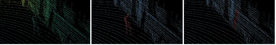
Although these systems lead to very complete 3D mapping of ur-ban scenes by capturing optical and 3D details (pavements, walls, trees, etc.), they often acquire mobile objects that are not persis-tent to the scene. This often happens in urban environments with objects such as cars, pedestrians, traffic cones, etc. As LiDAR sensors cannot penetrate through opaque objects, those mobile objects cast shadows behind them where no point has been ac-quired (Figure 1, left). Therefore, merging optical data with the point cloud can be ambiguous as the point cloud might repre-sent objects that are not prerepre-sent in the optical image. Moreover, these shadows are also largely visible when the point cloud is not viewed from the original acquisition point of view. This might
Figure 1. One result of our proposed method. (left) original point cloud, (center) segmentation, (right) disocclusion. end up being distracting and confusing for visualization. Thus, the segmentation of mobile objects and the reconstruction of their background remain a strategic issue in order to improve the un-derstability of urban 3D scans. We refer to this problem as disoc-clusion in the rest of the paper.
In real applicative contexts, we acknowledge that the disoccluded regions might cause a veracity issue for end-users so that the re-construction masks should be kept in the metadata. Using these masks, further processing steps may then choose to process dif-ferently disoccluded regions (e.g. kept for artefact-free visualiza-tions or discarded during object extracvisualiza-tions).
We argue that working on simplified representations of the point cloud, especially range images, enables specific problems such as disocclusion to be solved not only using traditional 3D techniques but also using techniques brought by other communities (image processing in our case).
The paper is organized as follows: after a review on related state-of-the-art, we detail how the point cloud is turned into a range im-age. In section 3, both segmentation and disocclusion aspects of the framework are explained. We then validate these approaches on different urban LiDAR data. Finally a conclusion and an open-ing are drawn.
2. RELATED WORKS
The growing interest for MMS over the past decade has lead to many works and contributions for solving problems of segmen-tation and disocclusion. In this part, we present a state-of-the-art on both segmentation and disocclusion.
2.1 Point cloud segmentation
The problem of point cloud segmentation has been extensively addressed in the past years. Three types of methods have emerged: geometry-based techniques, statistical techniques and techniques based on simplified representations of the point cloud.
Geometry-based segmentation The first well-known method in this category is region-growing where the point cloud is seg-mented into various geometric shapes based on the neighboring area of each point (Huang and Menq, 2001). Later, techniques that aim at fitting primitives (cones, spheres, planes, cubes ...) in the point cloud using RANSAC (Schnabel et al., 2007) have been proposed. Others look for smooth surfaces (Rabbani et al., 2006). Although those methods do not need any prior about the number of objects, they often suffer from over-segmenting the scene and as a result objects are segmented in several parts.
Statistical segmentation The methods in this category analyze the point cloud characteristics (Demantke et al., 2011, Weinmann et al., 2015, Br´edif et al., 2015). They consider different prop-erties of the PCA of the neighborhood of each point in order to perform a semantic segmentation. It leads to a good separation of points that belongs to static and mobile objects, but not to the distinction between different objects of the same class.
Simplified model for segmentation MMS LiDAR point clouds typically represent massive amounts of unorganized data that are difficult to handle, different segmentation approaches based on a simplified representation of the point cloud have been proposed. (Papon et al., 2013) proposes a method in which the point cloud is first turned into a set of voxels which are then merged using a variant of the SLIC algorithm for super-pixels in 2D images (Achanta et al., 2012). This representation leads to a fast segmentation but it might fail when the scale of the ob-jects in the scene is too different. Another simplified model of the point cloud is presented by (Zhu et al., 2010). The authors take advantage of the implicit topology of the sensor to repre-sent the point cloud as a 2-dimensional range image in order to segment it before performing classification. The segmentation is done through a graph-based method as the notion of neighbor-hood is easily computable on a 2D image. Although the provided segmentation algorithm is fast, it suffers from the same issues as geometry-based algorithms such as over-segmentation or inco-herent segmentation. Moreover, all those categories of segmen-tation techniques are not able to treat efficiently both dense and sparse LiDAR point cloudse.g.point clouds aquired with high or low sampling rates compared to the real-world feature sizes. In this paper, we present a novel simplified model for segmentation based on histograms of depth in range images.
2.2 Disocclusion
Disocclusion of a scene has only been scarcely investigated for 3D point clouds (Sharf et al., 2004, Park et al., 2005, Becker et al., 2009). These methods mostly work on complete point clouds rather than LiDAR point clouds. This task, also referred to as inpainting, has been much more studied in the image pro-cessing community. Over the past decades, various approaches have emerged to solve the problem in different manners. Patch-based methods such as (Criminisi et al., 2004) (and more re-cently (Buyssens et al., 2015b, Lorenzi et al., 2011)) have proven their strengths. They have been extended for RGB-D images (Buyssens et al., 2015a) and to LiDAR point clouds (Doria and Radke, 2012) by considering an implicit topology in the point cloud. Variational approaches represent another type of inpaint-ing algorithms (Chambolle and Pock, 2011, Bredies et al., 2010, Weickert, 1998, Bertalmio et al., 2000). They have been extended to RGB-D images by taking advantage of the bi-modality of the data (Ferstl et al., 2013, Bevilacqua et al., 2017). Even if the results of the disocclusion are quite satisfying, those models re-quire the point cloud to have color information as well as the 3D data. In this work, we introduce an improvement to a variational disocclusion technique by taking advantage of a horizontal prior.
3. METHODOLOGY
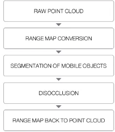
The main steps of the proposed framework, from the raw point cloud to the final result, are described in Figure 2. We detail each of these steps in this section.
Figure 2. Overview of the proposed framework.
3.1 Range maps and sensor topology
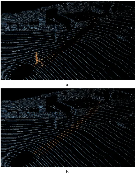
Figure 3. Example of a point cloud from the KITTI database (top) turned into a range image (bottom). Note that the black
area in (b) corresponds to pulses with no returns.
number of consecutive scanlines and thus a temporal dimension. 3D LiDAR sensors are based on multiple simultaneous scanline acquisitions (e.g. H = 64) such that scanlines may be stacked horizontally to form an image, as illustrated in Figure 3.
Whereas LiDAR pulses are emitted somewhat regularly, many pulses yield no range measurements due, for instance, to reflec-tive surfaces, absorption or absence of target objects (e.g. in the sky direction). Therefore the sensor topology is only a relevant approximation for emitted pulses but not for echo returns, such that the range image is sparse with undefined values where pulses measured no echoes. Considering echo datasets as a multi-layer depth image is beyond the scope of this paper.
The sensor topology only provides an approximation of the im-mediate 3D point neighborhoods, especially if the sensor moves or turns rapidly compared to its sensing rate. We argue however that this approximation is sufficient for most purposes, as it has the added advantage of providing pulse neighborhoods that are reasonably local both in terms of space and time, thus being ro-bust to misregistrations, and being very efficient to handle (con-stant time access to neighbors). Moreover, as LiDAR sensor de-signs evolve to higher sampling rates within and/or across scan-lines, the sensor topology will better approximate spatio-temporal neighborhoods, even in the case of mobile acquisitions.
We argue that raw LiDAR datasets generally contain all the infor-mation (scanline ordering, pulses with no echo, number of points per turn...) to enable a constant-time access to a well-defined implicit sensor topology. However it sometimes occurs that the dataset received further processings (points were reordered or fil-tered, or pulses with no return were discarded). Therefore, the sensor topology may only be approximated using auxilliary point attributes (time,θ,φ, fiber id...) and guesses about acquisition settings (e.g. guessing approximate∆time values between suc-cessive pulse emissions).
In the following sections, the range image is denoteduR.
3.2 Point cloud segmentation
We now propose a segmentation technique based on range his-tograms. For the sake of simplicity, we assume that the ground is relatively flat and remove ground points by plane fitting.
Instead of segmenting the whole range imageuR directly, we first split this image inS sub-windowsuRs, s= 1. . . Sof size
a. b.
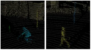
Figure 4. Result of the histogram segmentation using (Delon et al., 2007). (a) segmented histogram (bins of 50cm), (b) result in
the range image using the same colors.
Figure 5. Example of point cloud segmentation using our model on various scenes.
Ws×H along the horizontal axis. For eachuRs, a depth
his-togramhs of B bins is built. This histogram is automatically
segmented intoCs classes using the a-contrario technique
pre-sented in (Delon et al., 2007). This technique presents the advan-tage of segmenting a 1D-histogram without any prior assumption, e.g. the underlying density function or the number of objects. Moreover, it aims at segmenting the histogram following an ac-curate definition of an admissible segmentation, preventing over and under segmentation from appearing. Examples of segmented histograms are given in Figure 4.
Once the histogram of successive sub-images have been seg-mented, we merge together the corresponding classes by check-ing the distance between each of their centroids. Let us define the centroid of the ithclassCi
sin the histogramhsof the sub-image
uR
wherebare all bins belonging to classCi
s. The distance between
two classesCsiandCrj, of two consecutive windows can be
de-CsiandCrjshould be merged. Results of this segmentation
pro-cedure can be found in Figure 5. We argue that the choice of
Ws, B andτ mostly depends on the type of data that is being
treated (sparse or dense). For sparse point clouds,B has to re-main small (e.g. 50) whereas for dense point clouds, this value can be increased (e.g. 200). In practice, we found out that good segmentations may be obtained on various kind of data by setting
Ws= 0.5×Bandτ= 0.2×B. Note that the windows are not
3.3 Disocclusion
The segmentation technique introduced above provides masks for the objects that require disocclusion. As mentioned in the begin-ning, we propose a variational approach to the problem of dis-occlusion of the point cloud. The Gaussian diffusion algorithm provides a very simple algorithm for the disocclusion of objects in 2D images by solving partial differential equations. This tech-nique is defined as follows:
∂u
∂t −∆u= 0inΩ×(0, T)
u(0, x) =u0(x)inΩ (3)
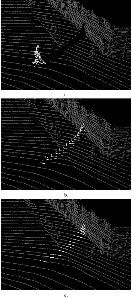
havinguan image defined onΩ,tbeing a time range and∆the Laplacian operator. As the diffusion is performed in every direc-tion, the result of this algorithm is often very smooth. Therefore, the result in 3D lacks of coherence as shown in Figure 7.b.
In this work, we assess that the structures that require disocclu-sion are likely to evolve smoothly along thexW andyW axis of
the real world as defined in Figure 6. Therefore, we set~ηfor each pixel to be a unitary vector orthogonal to the projection of
zW in theuRrange image. This vector will define the direction
in which the diffusion should be done to respect this prior. Note that most of MLS systems provide georeferenced coordinates of each point that can be used to define~η.
We aim at extending the level lines ofualong~η. This can be expressed ash∇u, ~ηi = 0. Therefore, we define the energy
F(u) = 1
2(h∇u, ~ηi) 2
. The disocclusion is then computed as a solution of the minimization probleminfuF(u). The gradient
of this energy is given by∇F(u) = −h(∇2
u)~η, ~ηi = −u~η~η,
whereu~η~ηstands for the second order derivative ofuwith
re-spect to~ηand∇2
ufor the Hessian matrix. The minimization of
Fcan be done by gradient descent. If we cast it into a continuous framework, we end up with the following equation to solve our disocclusion problem:
∂u
∂t −u~η~η= 0inΩ×(0, T)
u(0, x) =u0(x)inΩ (4)
using previously mentioned notations. We recall that ∆u =
u~η~η+u~ηT~ηT, where~ηT stands for a unitary vector orthogonal to~η. Thus, Equation (4) can be seen as an adaptation the Gaus-sian diffusion equation (3) to respect the diffusion prior in the direction~η. Figure 7 shows a comparison between the original Gaussian diffusion algorithm and our modification. The Gaus-sian diffusion leads to an over-smoothing of the scene, creating an aberrant surface whereas our modification provides a result that is more plausible.
Figure 6. Definition of the different frames between the LiDAR sensor (xL,yL,zL) and the real world (xW,yW,zW).
a.
b.
c.
Figure 7. Comparison between disocclusion algorithms. (a) is the original point cloud (white points belong to the object to be disoccluded), (b) the result after Gaussian diffusion and (c) the
The equation proposed in (4) can be solved iteratively. The num-ber of iterations simply depends on the size of the area that needs to be filled in.
3.4 Range image to 3D point cloud
After the segmentation and the disocclusion, we need to turn the range image back to the 3D space. For every point pi of the
original point cloud, we definepo
i andpei respectively the point
of emission and the point of echo ofpi. We denotedorig(pi)the
original range ofpianddrec(pi)its range after disocclusion. The
new coordinatespf inali of each point can be obtained using the
following formula:
The range image can then be easily turned back to a 3D point cloud while including the disocclusion.
4. RESULTS
In this part, the results of the segmentation of various objects and the disocclusion of their background are detailed.
4.1 Sparse point cloud
A first result is shown in Figure 8. This result is obtained for a sparse point cloud (≈106
pts) of the KITTI database (Geiger et al., 2013). A pedestrian is segmented out of the scene using our proposed segmentation technique. The segmentation result is used as a mask for the disocclusion of its background using our modified variational technique for disocclusion. Figure 8.a shows the original range image. In Figure 8.b, the dark region corresponds to the result of the segmentation step on the pedes-trian. For practical purpose, a very small dilatation is applied to the mask (radius of 2px in sensor topology) to ensure that no outlier points (near the occluder’s silhouette with low accuracy or on the occluder itself) bias the reconstruction. Finally, Fig-ure 8.c shows the range image after the reconstruction. We can see that the disocclusion performs very well as the pedestrian has completely disappeared and the result is visually plausible in the range image.
In this scene,~ηhas a direction that is very close to thexaxis of the range image and the 3D point cloud is acquired using a panoramic sensor. Therefore, the coherence of the reconstruc-tion can be checked by looking how the acquisireconstruc-tion lines are con-nected. Figure 9 shows the reconstruction of the same scene in 3 dimensions. We can see that the acquisition lines are properly retrieved after removing the pedestrian. This result was generated in 4.9 seconds using Matlab on a 2.7GHz processor. Note that a similar analysis can be done on the results presented in Figure 1.
a. b. c.
Figure 8. Result of disocclusion on a pedestrian on the KITTI database (Geiger et al., 2013). (a) is the original range image, (b)
the segmented pedestrian (dark), (c) the final disocclusion. Depth scale is given in meters.
a.
b.
Figure 9. Result of the disocclusion on a pedestrian in 3D. (a) is the original mask highlighted in 3D, (b) is the final
reconstruction.
4.2 Dense point cloud
In this work, we aim at presenting a model that performs well on both sparse and dense data. Figure 10 shows a result of the disocclusion of a car in a dense point cloud. This point cloud was acquired using the Stereopolis-II system (Paparoditis et al., 2012) and contains over4.9million points. In Figure 10.a, the original point cloud is displayed with the color based on the reflectance of the points for a better understanding of the scene. Figure 10.b highlights the segmentation of the car using our model, dilated to prevent aberrant points. Finally, Figure 10.c depicts the result of the disocclusion of the car using our method.
We can note that the car is perfectly removed from the scene. It is replaced by the ground that could not have been measured during the acquisition. Although the reconstruction is satisfying, some gaps are left in the point cloud. Indeed, in the data used for this example, pulse returns with large deviation values were discarded. Therefore, the windows and the roof of the car are not present in the point cloud before and after the reconstruction as no data is available.
4.3 Quantitative analysis
a.
b.
c.
Figure 10. Result of the disocclusion on a car in a dense point cloud. (a) is the original point cloud colorized with the reflectance, (b) is the segmentation of the car highlighted in
orange, (c) is the result of the disocclusion.
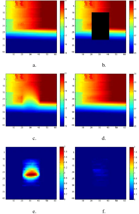
The test was done on 20 point clouds in which an area was manu-ally removed and then reconstructed. After that, we computed the MAE (Mean Absolute Error) between the ground truth and the reconstruction (where the occlusion was simulated) using both Gaussian disocclusion and our model. We recall that the MAE is expressed as follows:
MAE(u1, u2) =
1
N
X
i,j∈Ω
|u1(i, j)−u2(i, j)| (6)
where u1, u2 are images defined onΩ withN pixels. Table
1 sums up the result of our experiment. We can note that our method provides a great improvement compared to the Gaussian disocclusion, with an average MAE lower than3cm. This result is largely satisfying as most of the structures to reconstruct were
Table 1. Comparison of the average MAE (Mean Absolute Error) on the reconstruction of occluded areas.
Gaussian Proposed model
Average MAE (meters) 0.591 0.0279 Standard deviation of MAEs 0.143 0.0232
a. b.
c. d.
e. f.
Figure 11. Example of results obtained for the quantitative experiment. (a) is the original point cloud (ground truth), (b) the
artificial occlusion in dark, (c) the disocclusion result with the Gaussian diffusion, (d) the disocclusion using our method, (e) the Absolute Difference of the ground truth against the Gaussian diffusion, (f) the Absolute Difference of the ground truth against
our method. Scales are given in meters.
situated from 12 to 25 meters away from the sensor.
Figure 11 shows an example of disocclusion following this pro-tocole. The result of our proposed model is visually very plau-sible whereas the Gaussian diffusion ends up oversmoothing the reconstructed range image which increases the MAE.
5. CONCLUSION
Considering the range image derived from the sensor topology enabled a simplified formulation of the problem from having to determine an unknown number of 3D points to estimating only the 1D depth in the ray directions of a fixed set of range im-age pixels. Beyond simplifying drastically the search space, it also provides directly a reasonable sampling pattern for the re-constructed point set.
Although the average results of the method are more than accept-able, it can underperform in some specific cases. Indeed, the seg-mentation step first relies on the good extraction of non-ground points, which can be tedious when the data quality is low. More-over, when the object that needs to be removed from the scene is hiding complex shapes, the disocclusion step can fail recovering all the details of the background and the result ends up being too smooth. This is likely to happen when disoccluding very large objects.
In the future, we will focus on improving the current model to perform better reconstruction by taking into account the neigh-borhood of the background of the object to remove either by us-ing a variational method or by extendus-ing patch-based method.
6. ACKNOWLEDGEMENT
J-F. Aujol is a member of Institut Universitaire de France. This work was funded by the ANR GOTMI (ANR-16-CE33-0010-01) grant.
REFERENCES
Achanta, R., Shaji, A., Smith, K., Lucchi, A., Fua, P. and S¨usstrunk, S., 2012. SLIC superpixels compared to state-of-the-art superpixel methods. IEEE Trans. on Pattern Analysis and Machine Intelligence.
Becker, J., Stewart, C. and Radke, R. J., 2009. LIDAR inpainting from a single image. In:IEEE Int. Conf. on Computer Vision.
Bertalmio, M., Sapiro, G., Caselles, V. and Ballester, C., 2000. Image inpainting. In:ACM Comp. graphics and interactive tech-niques.
Bevilacqua, M., Aujol, J.-F., Biasutti, P., Br´edif, M. and Bugeau, A., 2017. Joint inpainting of depth and reflectance with visibil-ity estimation. ISPRS Journal of Photogrammetry and Remote Sensing.
Bredies, K., Kunisch, K. and Pock, T., 2010. Total generalized variation.SIAM Journal on Imaging Sciences.
Br´edif, M., Vallet, B. and Ferrand, B., 2015. Distributed dimensionality-based rendering of LIDAR point clouds. Inter-national Archives of the Photogrammetry, Remote Sensing and Spatial Information Sciences.
Buyssens, P., Daisy, M., Tschumperl´e, D. and L´ezoray, O., 2015a. Depth-aware patch-based image disocclusion for virtual view synthesis. In:ACM SIGGRAPH.
Buyssens, P., Daisy, M., Tschumperl´e, D. and L´ezoray, O., 2015b. Exemplar-based inpainting: Technical review and new heuristics for better geometric reconstructions. IEEE Trans. on Image Processing.
Chambolle, A. and Pock, T., 2011. A first-order primdual al-gorithm for convex problems with applications to imaging. Jour. of Math. Imag. and Vis.
Criminisi, A., P´erez, P. and Toyama, K., 2004. Region filling and object removal by exemplar-based image inpainting.IEEE Trans. on Image Processing.
Delon, J., Desolneux, A., Lisani, J.-L. and Petro, A. B., 2007. A nonparametric approach for histogram segmentation. IEEE Trans. on Image Processing.
Demantke, J., Mallet, C., David, N. and Vallet, B., 2011. Di-mensionality based scale selection in 3D LIDAR point clouds. International Archives of the Photogrammetry, Remote Sensing and Spatial Information Sciences.
Doria, D. and Radke, R., 2012. Filling large holes in lidar data by inpainting depth gradients. In:Int. Conf. on Pattern Recognition.
El-Halawany, S., Moussa, A., Lichti, D. and El-Sheimy, N., 2011. Detection of road curb from mobile terrestrial laser scanner point cloud. In:Proceedings of the ISPRS Workshop on Laserscanning, Calgary, Canada., Vol. 2931.
Ferstl, D., Reinbacher, C., Ranftl, R., R¨uther, M. and Bischof, H., 2013. Image guided depth upsampling using anisotropic total generalized variation. In:IEEE Int. Conf. on Computer Vision.
Geiger, A., Lenz, P., Stiller, C. and Urtasun, R., 2013. Vision meets robotics: The KITTI dataset. International Journal of Robotics Research.
Goulette, F., Nashashibi, F., Abuhadrous, I., Ammoun, S. and Laurgeau, C., 2006. An integrated on-board laser range sensing system for on-the-way city and road modelling. International Archives of the Photogrammetry, Remote Sensing and Spatial In-formation Sciences.
Hervieu, A. and Soheilian, B., 2013. Semi-automatic road/pavement modeling using mobile laser scanning.ISPRS An-nals of the Photogrammetry, Remote Sensing and Spatial Infor-mation Sciences.
Hervieu, A., Soheilian, B. and Br´edif, M., 2015. Road marking extraction using a MODEL&DATA-DRIVEN Rj-Mcmc. ISPRS Annals of the Photogrammetry, Remote Sensing and Spatial In-formation Sciences.
Huang, J. and Menq, C.-H., 2001. Automatic data segmentation for geometric feature extraction from unorganized 3D coordinate points.IEEE Trans. on Robotics and Automation.
Lorenzi, L., Melgani, F. and Mercier, G., 2011. Inpainting strate-gies for reconstruction of missing data in VHR images. IEEE Trans. on Geoscience and Remote Sensing Letters.
Paparoditis, N., Papelard, J.-P., Cannelle, B., Devaux, A., So-heilian, B., David, N. and Houzay, E., 2012. Stereopolis II: A multi-purpose and multi-sensor 3D mobile mapping system for street visualisation and 3D metrology. Revue franc¸aise de pho-togramm´etrie et de t´el´ed´etection.
Papon, J., Abramov, A., Schoeler, M. and Worgotter, F., 2013. Voxel cloud connectivity segmentation-supervoxels for point clouds. In:IEEE Conf. on Computer Vision and Pattern Recog-nition.
Park, S., Guo, X., Shin, H. and Qin, H., 2005. Shape and appear-ance repair for incomplete point surfaces. In:IEEE Int. Conf. on Computer Vision, Vol. 2.
Schnabel, R., Wahl, R. and Klein, R., 2007. RANSAC based out-of-core point-cloud shape detection for city-modeling. Pro-ceedings of Terrestrisches Laserscanning”.
Serna, A. and Marcotegui, B., 2013. Urban accessibility diag-nosis from mobile laser scanning data. ISPRS Journal of Pho-togrammetry and Remote Sensing.
Sharf, A., Alexa, M. and Cohen-Or, D., 2004. Context-based surface completion.ACM Trans. on Graphics.
Weickert, J., 1998. Anisotropic diffusion in image processing. Vol. 1, Teubner Stuttgart.
Weinmann, M., Jutzi, B., Hinz, S. and Mallet, C., 2015. Seman-tic point cloud interpretation based on optimal neighborhoods, relevant features and efficient classifiers. ISPRS Journal of Pho-togrammetry and Remote Sensing.