Thermodynamics and constitutive theory for
multiphase porous-media flow considering
internal geometric constraints
William G. Gray
Department of Civil Engineering and Geological Sciences, University of Notre Dame, Notre Dame, IN 46556-0767, USA
(Received 24 February 1998; accepted 12 June 1998)
This paper provides the thermodynamic approach and constitutive theory for closure of the conservation equations for multiphase flow in porous media. The starting point for the analysis is the balance equations of mass, momentum, and energy for two fluid phases, a solid phase, the interfaces between the phases and the common lines where interfaces meet. These equations have been derived at the macroscale, a scale on the order of tens of pore diameters. Additionally, the entropy inequality for the multiphase system at this scale is utilized. The internal energy at the macroscale is postulated to depend thermodynamically on the extensive properties of the system. This energy is then decomposed to provide energy forms for each of the system components. To obtain constitutive information from the entropy inequality, information about the mechanical behavior of the internal geometric structure of the phase distributions must be known. This information is obtained from averaging theorems, thermodynamic analysis, and from linearization of the entropy inequality at near equilibrium conditions. The final forms of the equations developed show that capillary pressure is a function of interphase area per unit volume as well as saturation. The standard equations used to model multiphase flow are found to be very restricted forms of the general equations, and the assumptions that are needed for these equations to hold are identified.q1999 Elsevier Science Ltd. All rights reserved.
Keywords: porous media, thermodynamics, continuum mechanics, averaging theory,
geometry.
NOMENCLATURE
Aa surface area forming the boundary of the a phase
Aab surface area of
ab-interface
aa specific interfacial area of the boundary of thea phase (area per unit of system volume)
aab specific interfacial area ofab-interface (area per unit of system volume)
ba external supply of entropy to theaphase bab external supply of entropy to theabinterface bwns external supply of entropy to the wns common line bm tensor used to write the outline form of the entropy
inequality in eqn (39)
caab accounts for contribution to the energy of thea phase of theabinterface
caba accounts for contribution to the energy of theab interphase of theaphase
cabwns accounts for contributions to the energy of theab
interface of the wns common line
cwnsab accounts for contributions to the energy of the wns common line of theabinterface
da deformation rate tensor of anaphase dab deformation rate tensor of anabinterface dwns deformation rate tensor of a wns common line dm deformation rate tensor: phase (m¼a), interface
(m¼ab), or common line (m¼wns)
Ea internal energy ofaphase per mass ofaphase Eab internal energy ofabinterface per mass of ab
interface
Ewns internal energy of wns common line per mass of wns common line
q1999 Elsevier Science Ltd
Printed in Great Britain. All rights reserved 0309-1708/99/$ - see front matter
PII: S 0 3 0 9 - 1 7 0 8 ( 9 8 ) 0 0 0 2 1 - 9
ˆ
Ea internal energy of theaphase per unit volume of system
ˆ
Eab internal energy of theabinterface per unit volume of system
ˆ
Ewns internal energy of the wns common line per unit volume of system
Ea extensive internal energy of thea phase
Eab extensive internal energy of theab interface
Ewns extensive internal energy of the wns common line Es Lagrangian strain tensor of the solid phase ˆ
eaab rate of transfer of mass fromab-interface to the a-phase
ˆ
eabwns rate of transfer of mass from wns common line to
theab-interface
em term accounting for the multipliers of velocity in outline entropy inequality (39)
Fs displacement vector of the solid phase ga external supply of momentum to thea phase gab external supply of momentum to theab interface gwns external supply of momentum to the wns common
line
ha external supply of energy to theaphase hab external supply of energy to theabinterface hwns external supply of energy to the wns common line I identity tensor
Jss average curvature of the solid surface calculated
with nspositive
Jaba average curvature of theab calculated with na positive
j jacobian of the motion of the solid phase
L material coefficients (with various superscripts and subscripts)
Lwns common line length
lwns specific length of wns common line (length per unit volume of medium)
Ma mass ofa phase
Mab mass ofab interface
Mwns mass of wns common line
na unit vector normal to and pointing outward from the surface of the aphase
p unit vector in direction of average principal cur-vature of the wns common line
pa pressure ofa-phase ˆ
Qaab energy transferred to thea-phase from theab -interface
ˆ
Qabwns energy transferred to theab-interface from the wns
common line
q effective total heat conduction vector qa heat conduction vector for theaphase qab heat conduction vector for theab interface qwns heat conduction vector for the wns common line
Sa entropy of theaphase
Sab entropy of theabinterface
Swns entropy of the wns common line
sa saturation of thea-phase, volume fraction of void space occupied by fluid phasea
ˆ
Taab force exerted on thea-phase by the ab-interface ˆ
Tabwns force exerted on theab-interface by the wns common line
ta stress tensor for theaphase tab stress tensor for theab interface twns stress tensor for the wns common line u velocity of a common line
Va volume of
a-phase
Vs
0 reference volume of solid phase
va velocity of theaphase vab velocity of theabinterface vwns velocity of the wns common line
va,ab velocity of theaphase relative to the velocity of theabinterface, va¹vab
vab,wns velocity of theabinterface relative to the velocity of the wns common line, vab¹vwns
w velocity of an interface
Xs reference position of a solid phase ‘particle’ x spatial position of a solid phase ‘particle’
xnss fraction of the solid phase surface in contact with
the non-wetting phase
xwss fraction of the solid phase surface in contact with
the wetting phase
Greek symbols
gab surface tension ofab-interface gwns lineal tension of wns-common line e porosity of the medium
ea volume fraction ofa-phase
ˆha entropy ofaphase per unit volume of system ˆhab entropy ofabinterface per unit volume of system ˆhwns entropy of wns common line per unit volume of
system v temperature
va temperature of theaphase vab temperature of theab interface vwns temperature of the wns common line va,ab temperature difference,va¹vab vab,wns temperature difference,vab¹vwns
k average principal curvature of the common line kn average normal curvature of the common line with
respect to the s surface
kwsg average geodesic curvature of the common line
with respect to the ws surface
l unit vector tangent to the wns common line ma chemical potential of theaphase
mab chemical potential of theabinterface mwns chemical potential of the wns common line nab unit vector on the common line normal toland
tangent to theabinterface
ra density ofaphase, mass ofaphase per volume of aphase
rab density ofab interface, mass ofabinterface per area ofabinterface
js stress in the solid due to deformation
jas stress in thea–solid interface due to solid defor-mation
t quantities defined in the text (with subscripts and superscripts) that are zero at equilibrium
F average contact angle between the w and s phases fa entropy conduction vector of theaphase
fab entropy conduction vector of theabinterface fwns entropy conduction vector of the wns common
line
ˆ
Qa grand canonical potential of thea phase per unit volume of system
ˆ
Qab grand canonical potential of theab interface per unit volume of system
ˆ
Qwns grand canonical potential of the wns common line per unit volume of system
Special symbols
Da=Dt material time derivative following the motion in
thea phase,]=]tþva·=
Dab=Dt material time derivative following the motion in
theab interface,]=]tþvab·=
Dwns=Dt material time derivative following the motion in
the wns common line,]=]tþvwns·=
P
bÞa summation over all phases excepta-phase = gradient operator with respect to spatial
coordinates
=X gradient operator with respect to reference coordinates
Superscripts and subscripts n non-wetting phase s solid phase w wetting phase
ns non-wetting–solid interface wn wetting–non-wetting interface ws wetting–solid interface
1 INTRODUCTION
Accurate description of multiphase flow in porous media requires that a number of system intricacies be accounted for. These include the presence of juxtaposed phases and their interfaces, the complicated geometry of pores, fluid dynamics giving rise to appearance and disappearance of interfaces, pendular rings of a wetting phase, ganglia of the non-wetting phase, and the behavior of films. A variety of forces, due to viscous effects, gravity, interfacial tension, and pressure are simultaneously present and influencing system behavior. A fundamental question in modeling the flow of fluids in porous media is how much detail should be included in such models. In virtually all laboratory and field scale models, microscale details (i.e., pore geometry and flow variations within those pores) are impossible to include
and are not actually needed. However, manifestation of those details at the macroscale (a scale involving tens to hundreds of pores) must be preserved. Traditionally, porosity and fluid saturations, concepts that do not exist at the microscale, are included in macroscale porous media theories to account for the presence of multiple phases at a point in a macroscale continuum. However, these addi-tional variables have proven insufficient to account for all important microscale processes that influence macroscale behavior. Because of the dynamic motion of the fluids, many configurations and distributions of the fluids are possible for a given saturation. Even at equilibrium, different distributions of fluids could exist at a prescribed saturation such that the balances of forces on the fluid are satisfied.
This matter has received attention in recent years and thermodynamic theories have been developed wherein interfacial effects are explicitly included.10,18,20,26,27 In these theories, in addition to porosity and saturation, specific interfacial area, the amount of interfacial area between two phases per unit volume of the system, is introduced as a macroscale independent variable. This variable is of impor-tance in studies of mass transfer among phases of a porous medium and thus is of wide interest. A number of proce-dures involving network models and experimental methods have been developed for measurement of interfacial areas.13,36,40,43
Porous media systems that involve flow of two or more fluids may also have common lines, curves formed in those instances when three different interface types come together. The common lines may play an important role in the movement of fluids and interfaces. Indeed, in a capillary tube where a meniscus between fluids is at rest, flow can be initiated only if the balance of forces on the common line, as well as the balance on the phases and the meniscus, is per-turbed. Thus, the question arises as to how the presence of common lines and the thermodynamic properties of those lines affect the macroscale flow processes in porous media. This question, and more general questions regarding the degree of detail that must be incorporated into macroscale theories, can be investigated only if appropriate conserva-tion equaconserva-tions for the common lines are available. Subse-quent to the development of a general theory, information obtained from experiments and observations may be used to evaluate the relative significance of various phenomena accounted for in the theory. At that point, simplifications can be made that eliminate unimportant terms from the modeling process. It is important to observe that by starting from a general formulation, one is forced to make explicit assumptions to arrive at equations to be used in a modeling exercise. Then, if the exercise proves unsuccessful, the source of the difficulty will lie in the approximations made. If, on the other hand, one begins with simple equa-tions based on empirical or intuitive ideas, the cause of the failure of such equations cannot be inferred.
procedure for developing usable equations for the simula-tion of multiphase subsurface flow involves six steps:
• Derivation of conservation equations for phases, interfaces, and common lines at the porous media scale, the macroscale, and of the entropy inequality for the system. Work to do this has been ongoing for many years. Initially, the work considered only phases; and balance laws studied were restricted to conservation of mass and momentum, e.g. Ref.47. The dissertation of Hassanizadeh22and the papers by Hassanizadeh and Gray23–25employed an averaging theory that extended this approach to inclusion of the energy equation and entropy inequality. Subse-quent to this, Gray and Hassanizadeh18 developed averaging theorems for interfaces and developed conservation relations for the interface properties as well. Finally, theorems for averaging over common lines were developed by Gray et al.21and have been employed in a paper by Gray and Hassa-nizadeh20. This latter reference, in fact, presents the set of averaged equations of mass, momentum, and energy conservation for phases, interfaces, and common lines that form the basis for a general study of multiphase flow.
• Postulation of thermodynamic dependences of the energy on independent variables for phases, inter-faces, and common lines and incorporation of these postulates into the entropy inequality. This task is one that has not, heretofore, been addressed thoroughly for macroscale system representation. There is a need to ensure that the fundamental ideas of thermodynamics are not neglected when making use of the principles of continuum mechanics. Note that classical thermodynamics deals with equilibrium systems only while con-tinuum mechanics deals with both equilibrium states and the transitions when a system is not at equilibrium. Nevertheless, it is important that the continuum mechanical description reduce to the classical thermodynamic one at steady state. Thermodynamics requires that consistent and systematic postulates be made concerning the dependence of internal energy on independent vari-ables. The presence of interfaces adds the compli-cation of excess surface properties such as mass per unit area and interfacial tension that must be accounted for in a conceptually and quantitatively consistent manner (surface excess properties from a microscale Gibbsian perspective are discussed, for example, in Miller and Neogi34and Gaydos et al.17). Then, from the postulated forms, relations among variables and insights into system behavior can be obtained. One of the most useful approaches for postulating the thermodynamic dependence of internal energy is the approach advocated in Callen12 and Bailyn9 and, used to advantage by
Gaydos et al.17in a study of microscopic capillarity, whereby the extensive energy is considered to be a function of the extensive variables of the system. With this approach, confusion about differences among Helmholtz potential, Gibbs potential, grand canonical potential, and enthalpy are diminished as they are simply mathematical rearrangements of the original postulated form for internal energy. Insights gained from applying microscale-based thermodynamic postulates to multiphase systems (e.g. Refs 1–4,15,34,35,37) are extremely valuable in formulating a macroscale theory, but do not replace the need for formulation of that theory in terms of macroscale variables. To develop the macroscale thermodynamics, the postulative approach of Callen12 will be employed after extension to the macroscale perspective. The philosophy of Callen12 is employed herein to obtain thermo-dynamic relations that are appropriate for a macro-scale description of a porous media system. One important point is that from the perspective of the macroscale, the system is composed of coexisting phases at a point and not juxtaposed phases, inter-faces, and common lines. Thus, in fact, the energy postulate should be made in terms of all compo-nents. The decomposition of the internal energy for the total system to the component parts describ-ing each phase, interface, and common line must be undertaken with caution.
• Determination of mechanical equilibrium con-straints and their incorporation into the entropy inequality. Although the geometric variables including porosity, saturation, areas per volume, and common line length per volume are indepen-dent variables, their deviations around an equili-brium state are not (e.g., a change in saturation of one fluid would be expected to cause a change in the amount of area bounding that fluid). These con-siderations give rise to employment of the aver-aging theorems to obtain relations among changes in geometric variables. These relations are useful in deriving both thermodynamic equilibrium condi-tions and dynamic relacondi-tions between changes in geometric variables and the thermodynamic state of the system.
constitutive functions in a systematic manner that is based on the second law of thermodynamics. The procedure of Coleman and Noll14 was applied to single phase systems to assure that the second law of thermodynamics is not violated by constitutive assumptions. Complementing this work are exten-sions and variations that consider multiphase mix-tures and interfaces (e.g., Refs19,25,38,45). Here, the macroscale entropy inequality will be exploited while taking into account constraints obtained from the geometric relations.
• Linearization of some of the constitutive functions to obtain conservation equations with their coeffi-cients capable of modeling dynamic systems. Although the localization theory for a three phase system provides 35 balance equations of mass, momentum, and energy for the phases, interfaces, and common lines, it also contains 150 constitutive functions that must be specified. The dependence of these functions on other system parameters are obtained under some assumptions. Also, the func-tional forms of the dependences of the stress tensors are obtained. However, in general, the actual func-tional relations between the constitutive functions and their independent variables are not known except at equilibrium. For example, at equilibrium the heat conduction vector is zero; but the general functional representation of this vector in terms of independent variables is not known at an arbitrary state of disequilibrium. Thus a compromise must be employed whereby functional forms are obtained ‘near’ equilibrium. Experimental and computational studies must subsequently be undertaken to deter-mine the definition of ‘nearness’. By this approach, which is similar to taking a Taylor series expansion of a function and ignoring higher order terms, results such as the heat conduction vector being proportional to the temperature gradient and a velocity proportional to a potential gradient are obtained. Because multiphase porous media flows are typically slow, they also satisfy the conditions of being ‘near enough’ to equilibrium that this linearization procedure provides relations appro-priate for many physical situations. It is important to note, however, that although the equations are linearized, the coefficients that arise still may have complex dependence on system parameters (e.g., relative permeability, which is traditionally simplified to be a function of saturation). Identifica-tion of those coefficients remains a challenging task.
• Determination of the physical interpretation of the coefficients, as possible, using geometric approxi-mations that provide insight into required labora-tory measurements. It is important that the theoretical procedure not simply be a propagator of unknown coefficients that have no chance of being measured or even understood. Therefore,
effort must be made to allow insightful study of the new coefficients through laboratory and com-puter experimentation. Thus, although a general formulation is employed, it is simplified to a manageable, yet still challenging, set of equations that can be effectively studied. As progress is made in parameterizing these systems, the approxima-tions employed can be relaxed so that more com-plex systems may be studied.
The first of the above steps was carried out by Gray and Hassanizadeh20for the general case including an arbitrary number of phases, interfaces, common lines, and common points. Here, the conservation equations developed in that paper will be simplified to the case of three phases (wetting phase w, non-wetting phase n, and solid phase s) prior to continuing the systematic approach to addressing thermo-dynamic and geometric issues. The result of this study is a ‘workable’ set of equations that arises from examination of a three-phase system, composed of a solid and two fluids. Additionally, the assumptions needed to reduce the general set of equations to the set traditionally used to model a three-phase system are made explicit.
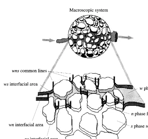
2 CONSERVATION EQUATIONS
Fig. 1 depicts a three-phase system consisting of a solid and two fluid phases, denoted by s, w, and n, respectively. The w phase will be referred to as the wetting phase because it preferentially wets the solid relative to the non-wetting n phase. The phases are separated by three different interfaces denoted as wn, ws, and ns where the paired indices refer to the phases on each side of the interface and the order of the indices is inconsequential. Additionally, a wns common line may exist. The three-phase system is a simplification of a more general case involving more phases in that no common points exist. General macroscale equations describing conservation of mass, momentum, and energy for phases and interfaces have been developed pre-viously.18,23 These have been collected, and equations for common lines and common points have been derived along with the entropy inequality for the system.20Here, these will be simplified to the forms needed to describe a three-phase system. The reduction to the required forms is a straightfor-ward manipulation of the general forms with the main dif-ferences being that summations over common lines reduce to terms involving the single common line and terms relat-ing to transfer processes at common points are zero since no common points exist for a three-phase system.
In addition, for convenience rather than necessity, the energy densities will be expressed per unit mass and per unit of system volume. Therefore, with Eabeing the internal energy of the a phase per unit mass of a phase, Eˆa will indicate the a phase energy per unit volume of porous medium. These two energy densities are related by
ˆ
energy of theabinterface per unit mass of interface while ˆ
Eab¼rabaabEabis the excess energy per unit volume of the system. Finally, the common line energy per unit mass of common line is denoted as Ewns while the common line internal energy per unit volume of the system is
ˆ
Ewns¼rwnslwnsEwns. Note that in the case of massless inter-faces and common lines, the energies per unit volume are still directly meaningful functions, while the product of mass density times energy per mass must be evaluated in the limit as the density approaches zero.
The objective of this section is to provide the needed balance equations rather than reproduce their derivation from the earlier general work.20
2.1 Phase conservation equations
The balance equations for the three-phase system are essen-tially unchanged from the general case with more phases. For the current study, each phase may have two different kinds of interfaces at its boundary. For example, the phase is bounded by some combination of wn and ws interfaces. The balance equations for the phases are as follows:
Macroscale mass conservation for thea-phase
Da(eara) Dt þe
a
ra=·va¼ X
bÞa
ˆ
eaab a¼w,n,s (1)
Macroscale momentum conservation for thea-phase
earaD
ava
Dt ¹=·(e
ata)¹earaga¼ X
bÞa
ˆ
Taab a¼w,n,s
(2)
Macroscale energy conservation for thea-phase
DaEˆa Dt ¹=·(e
aqa)¹(
eata¹EˆaI):=va¹earaha
¼Ea X
bÞa
ˆ
eaabþ X
bÞa
ˆ
Qaab a¼w,n,s ð3Þ
The terms on the right side of the equations account for exchanges with the bounding interfaces. The complete notation used is provided at the beginning of the text.
2.2 Interface conservation equations
These equations express conservation of mass, momentum, and energy of the interface. The interfaces may exchange properties with adjacent phases and with the common line. The balance equations are as follows:
Macroscale mass conservation for theab-interface
Dab(aabrab) Dt þa
ab
rab=·vab¼ ¹(eˆaabþeˆbab)þeˆabwns
ab¼wn,ws,ns ð4Þ
Macroscale momentum conservation for theab-interface
aabrabD
abvab
Dt ¹=·(a
abtab)¹aab
rabgab
¼ ¹ X
i¼a,b
(eˆiabvi,abþTˆ
i
ab)þTˆ ab
wns ab¼wn,ws,ns
ð5Þ
Macroscale energy conservation for theab-interface
DabEˆab Dt ¹=·(a
abqab)¹(aabtab¹Eˆab
I):=vab¹aabrabhab
¼ ¹ X
i¼a,b
{eˆiab[Eiþ(vi,ab)2=2]þTˆi
ab·v
i,abþQˆi
ab}
þEabeˆabwnsþQˆ
ab
wns ð6Þ
2.3 Common line conservation equations
The balance equations for the common line account for the properties of the common line and the exchange of those properties with the interfaces that meet to form the common line. The appropriate equations for the case where there are three phases, and thus only one common line and no com-mon points, are as follows.
Macroscale mass conservation for the wns-common line
Dwns(lwnsrwns)
Dt þl
wns
rwns=·vwns¼ ¹(eˆwnwnsþeˆ ws wnsþeˆ
ns wns)
(7) Fig. 1. Depiction of a three-phase system at a macroscale point
Macroscale momentum balance for the wns-common line
lwnsrwnsD
wns
vwns Dt ¹=·(l
wns
twns)¹lwnsrwnsgwns
¼ ¹ X
ij¼wn,ws,ns (eˆijwnsv
ij,wns
þTˆijwns) ð8Þ
Macroscale energy conservation for the wns-common line
DwnsEˆwns Dt ¹=·(l
wnsqwns)
¹(lwnstwns¹EˆwnsI):=vwns
¹lwnsrwnshwns
¼ ¹ X
ij¼wn,ws,ns
{eˆijwns[Eijþ(vij,wns)2=2ÿ þTˆijwns·vij,wnsþQˆijwns}
ð9Þ
2.4 Entropy inequality
An entropy inequality has been derived for each phase, interface, and the common line as discussed in Gray and Hassanizadeh.20 However, the entropy exchange terms between the different components prevent the individual inequalities from being particularly useful. The power of the entropy inequalities comes in calculating their sum such that the exchange terms cancel. The combined entropy inequality for the three phase system takes the form:
L¼X
a
Daˆha Dt þˆh
aI:=va¹=·(eafa)¹earaba
þX
ab
Dabˆhab Dt þˆh
abI:=vab¹=·(aabfab)
(
¹aabrabbab¹hab X
i¼a,b
ˆ eiab
) þD
wns
ˆhwns Dt
þˆhwnsI:=vwns¹=·(lwnsfwns)¹lwnsrwnsbwns
¹hwns X
ij¼wn,ws,ns
ˆ
eijwns$0 ð10Þ
3 IDENTIFICATION OF UNKNOWNS
For the conservation equations to be useful in an appli-cation, some determination must be made of the functional forms of the variables that appear in these equations. In fact, for the three phase system, there are a total of 35 conserva-tion equaconserva-tions (for each phase, interface, and common line there is one mass conservation equation, three momentum equations, and one energy equation). For these equations, the following 35 variables will be designated as primary
physical independent variables:
• 15 phase properties: rw, rn, rs, vw, vn, Fs, vw, vn, vs
• 15 interface properties: rwn,rws, rns, vwn, vws, vns, vwn,vws,vns
• 5 common line properties:rwns, vwns,vwns
In addition to these quantities, six primary geometric inde-pendent variables appear in the equations which account for the distributions of phases, interfaces, and common line in the system. These variables are:
• 6 geometric variables:e, sw, awn, aws, ans, lwns
It is important to note that the six dynamic geometric vari-ables, not present in a microscale formulation but arising at the macroscale, provide an excess of unknowns over and above the 35 primary variables that are associated with the 35 balance equations. The development of equations that describe the dynamics of the macroscale geometry is a sig-nificant challenge.
Finally, there are additional quantities appearing in the equation that must be expressed as constitutive functions of the physical and geometric variables. These quantities are:
• 75 functions from the phase equations: ˆ
Ea,ta,Tˆaab,qa,Qˆaab,ˆha,eˆaab,fa,ba;
a¼w,n,s; ab¼wn,ws,ns
• 60 functions from the interface equations: ˆ
Eab,tab,Tˆabwns,qab,Qˆabwns,ˆhab,eˆabwns,fab,bab;
ab¼ws,wn,ns
• 15 functions from the common line equation: ˆ
Ewns,twns,qwns,ˆhwns,fwns,bwns
Thus to close the system and have a set of equations that can be used to model the three phase system, there is a need for 150 constitutive functions of the physical properties and geometric variables, as well as the six additional relations among the geometric and physical parameters. The consti-tutive functions will be assumed to be expressible as func-tions of the 35 independent variables, the geometric variables, and gradients of some of these quantities.
Assumption I The 150 constitutive functions may be expressed in terms of the following set of independent variables:
z¼{rw,rn,rs,vw,vn,Fs,vw,vn,vs,e,sw,=vw,=vn,=vs,=e,
=sw,rwn,rws,rns,vwn,vws,vns,vwn,vws,vns,awn,aws,ans,
=vwn,=vws,=vns,=awn,=aws,=ans,rwns,vwns,vwns,
lwns,=vwns,=lwns} ð11Þ
be adequate for description of the porous media systems under study here. Should the resulting equations prove to be incapable of describing a process of interest, then it may be necessary to propose an expanded list of independent variables.
Determination of the constitutive functions such that the equation system may be closed is certainly a significant task, but one that can be accomplished with a combination of systematic thermodynamic postulates, reasonable geometric conditions, exploitation of the entropy inequality, and laboratory verification. The theoretical steps to be employed will be demonstrated next.
4 THERMODYNAMIC ASSUMPTIONS AND RELATIONS
One of the important challenges to obtaining a complete theory of multi-phase flow is the postulation of the appro-priate thermodynamics. Here, an approach is followed that is based on the key assumption:
Assumption II The dependence of energy of the phases, interfaces, and common lines on the independent variables is the same function whether or not the full multi-phase system is at equilibrium.
This assumption, which means that energy is a function of a subset of the independent variables in list (11), may limit the theory such that it applies only to slowly changing systems, but this is the case in most porous media flow situations. An advantageous consequence of this assumption is that some mathematically complex relations involving the dependence of energy on quantities such as velocity or tem-perature gradient which are of little physical consequence do not arise. The postulated dependences will be made with the total energy being dependent on extensive properties of the phases, interfaces, and common line. The postulates of dependence of energy on the physical and geometric vari-ables are made in a manner consistent with the philosophy of Callen12for microscopic systems but is more general.
4.1 System thermodynamics
For the system consisting of phases, interfaces, and the common line in which points are viewed from the macro-scale perspective, the energy is postulated to be a function of the entropies of the system components, the mass of each component, and the geometric extents such that:
E¼E(Sw,Sn,Ss,Swn,Sws,Sns,Swns,Mw,Mn,Ms,Mwn,
Mws,Mns,Mwns,Vw,Vn,V0sEs,Awn,Aws,Ans,Lwns):
ð12Þ
All variables written in script are extensive variables. Many useful relations describing the equilibrium thermodynamic behavior of the multiphase system as a whole may be
derived based on postulate (12). However, the goal of this work is to obtain a dynamic description of the multi-phase system at the macroscale and the contribution of each component of the system to the dynamic behavior. For example, when not at equilibrium, phases, interfaces, and common lines co-existing at a macroscopic point might not be at the same temperature. Therefore, to describe such a situation, it is necessary to decompose the functional form of the energy given by postulate (12) into its component parts at each macroscale point and treat those separately. The path to such a decomposition is not entirely obvious and certainly is not unique.
One necessary part of the decomposition is to require that the total system energy be equivalent to the sum of its com-ponent parts from the phases, interfaces, and common lines such that:
E¼EwþEnþEsþEwnþEwsþEnsþEwns: (13)
The next step is to determine the functional dependence of each of the seven components. The most general proposal for such dependence would be to allow each of the compo-nent energies to depend on the full list of extensive vari-ables of the system, as in eqn (12). Although this formulation is attractive because of its generality, it lacks appeal because it fails to dismiss negligible interactions among system components such that the system description obtained is unnecessarily complex from a mathematical perspective. Thus, an alternative more restrictive approach will be followed here for specifying the dependence of the energy on extensive variables that allows for some coupling of the thermodynamic properties of components, but not all possible couplings. It must be emphasized that this restric-tion may limit the general applicability of the theory, but it is proposed as a reasonable compromise among generality, the need to relate the theory to a real system, and the couplings that are expected to be important. The assump-tion that will be employed is as follows:
Assumption III A multiphase system is composed of phases, interfaces, and common lines which will be referred to as components. The total energy of each component will be assumed to be a function of the entropy of that compo-nent, the geometric extensive variable of that compocompo-nent, the mass of that component, and the geometric extensive variables of all microscopically adjacent components.
the average microscale distance between points in each component is small (e.g., in thin films or for highly dis-persed phases, interfaces and common lines). In addition, the functional dependences obtained by Assumption III must still lead to thermodynamic relations involving com-ponent properties consistent with the thermodynamic analysis of the system as a whole.
4.2 Constitutive postulates for phase energy functions
The dependence of energy of the fluid phases on their prop-erties is postulated as:
Ew¼EwÿSw,Vw,Mw,Awn,Aws
(14a)
En¼EnÿSn,Vn,Mn,Awn,Ans
(14b)
The solid phase energy depends on the state of strain of the solid9such that it is expressed as:
Es¼EsÿSs,Vs0Es,Ms,Aws,Ans
(14c)
The inclusion of a dependence on the interfacial areas in these expressions is a departure from the type of postulate made when a system is to be modeled at the microscale. This is to account for changes in energy that may occur when the amount of surface area per volume of phase is large. Additionally, note that the nature of a solid accounts for its energy being postulated as depending on the state of deformation rather than its volume. From these equations, because energy is a homogeneous first order function,9,12 the Euler forms of the energy are:
Ew¼vwSw¹pwVwþmwMwþcwwnAwnþcwwsAws (15a)
En¼vnSn¹pnVnþmnMnþcnwnAwnþcnnsAns (15b)
and
Es¼vsSs¹js:V0sEsþmsMsþcswsA ws
þcsnsA ns
(15c)
As an example, note that the partial derivative ofEw with respect to one of its independent variables, as listed in eqn (14a), is simply equal to the coefficient of that variable in eqn (15a). Similar observations apply for all the phase energies as well as the interface and common line energies to be discussed subsequently.
Now convert eqns (15a), (15b) and (15c) such that they are on a per unit system volume basis:
ˆ
Ew(ˆhw,ew,ewrw,awn,aws)
¼vwˆhw¹pwewþmwewrwþcwwnawnþcwwsaws (16a)
ˆ
En(ˆhn,en,enrn,awn,ans)
¼vnˆhn¹pnenþmnenrnþcnwna wn
þcnnsa ns
(16b)
ˆ Es ˆhs,e
s
Es j ,e
s
rs,aws,ans
¼vsˆhs¹js :esEs=jþmsesrsþcswsawsþcsnsans (16c)
Make use of the definition of the grand canonical potential:
ˆ
Qa¼Eˆa¹vaˆha¹maeara: (17)
and employ Legendre transformations on ˆha and eara to obtain:
ˆ
Qwÿvw,ew,mw,awn,aws¼ ¹pwewþcwwna wn
þcwwsa ws
(18a)
ˆ
Qnÿvn,en,mn,awn,ans
¼ ¹pnenþcwnn awnþcnnsans
(18b)
ˆ Qs ˆvs,e
s
Es j ,m
s,
aws,ans
¼ ¹js:esEs=jþcswsawsþcsnsans
(18c)
where
]Qˆa
]va¼ ¹ˆh
a (18d)
]Qˆa
]ea¼ ¹p
a
a¼w,n (18e)
]Qˆs
](esEs=j)¼ ¹j s
(18f)
]Qˆa
]ma¼ ¹e
ara (18g)
]Qˆa
]aab¼c
a
ab: (18h)
For eqns (16a), (16b) and (16c), it is also worth noting that their respective Gibbs–Duhem equations are:
0¼ˆhwdvw¹ewdpwþewrwdmwþawndcwwnþa ws
dcwws
(19a)
0¼ˆhndvn¹endpnþenrndmnþawndcnwnþa ns
dcnns
(19b)
and
0¼ˆhsdvs¹e
s
Es j : dj
s
þesrsdmsþawsdcswsþa ns
dcsns:
(19c)
4.3 Constitutive postulates for interfacial energy functions
The dependence of the internal energy of the interfaces on their properties are postulated as:
Ewn¼Ewn(Swn,Awn,Mwn,Vw,Vn,Lwns) (20a)
Ews¼Ews(Sws,Aws,Mws,Vw,Vs0Es,Lwns) (20b)
Here the common line length is included as an indicator of the length of the boundary of the interface, a measure of whether the microscale areas are small and distributed or large. The inclusion of the volumes of the adjacent fluid phases and the strain tensor of the adjacent solid phase adds generality that may be important when the amount of volume per area is small. The Euler forms of the energy equations are:
Ewn¼vwnSwnþgwnAwnþmwnMwn¹cwnw V w
¹cwnn V n
¹cwnwnsL wns
(21a)
Ews¼vwsSwsþgwsAwsþmwsMws¹cwswV w
¹jws:Vs0Es¹cwswnsLwns (21b)
Ens¼vnsSnsþgnsAnsþmnsMns¹cnsnVn
¹jns:Vs0Es¹cnswnsLwns (21c)
Conversion of these expressions to a per-unit-volume basis whereEˆab is the energy per unit volume of medium gives:
ˆ
Ewn¼Eˆwnÿˆhwn,awn,awnrwn,ew,en,lwns
¼vwnˆhwnþgwnawnþmwnawnrwn¹cwnw e w
¹cwnn e n
¹cwnwnsl wns
(22a)
ˆ
Ews¼Eˆwsÿˆhws,aws,awsrws,ew,esEs=j,lwns
¼vwsˆhwsþgwsawsþmwsawsrws¹cwswe w
¹jws:esEs=j¹cwswnslwns (22b)
ˆ
Ens¼Eˆnsÿˆhns,ans,ansrns,en,esEs=j,lwns
¼vnsˆhnsþgnsansþmnsansrns¹cnsne n
¹jns:esEs=j¹cnswnslwns (22c)
Make use of the definition of the grand canonical potential of the form:
ˆ
Qab¼Eˆab¹vabˆhab¹mabaabrab (23)
and Legendre transformation of the independent variables ˆhab and aabrab to obtain:
ˆ
Qwn(vwn,awn,mwn,ew,en,lwns)
¼gwnawn¹cwnw ew¹cwnn en¹cwnwnslwns (ð24aÞ
ˆ
Qws(vws,aws,mws,ew,esEs=j,lwns)
¼gwsaws¹cwswew¹jws:esEs=j¹cwswnslwns (24b)
ˆ
Qns(vns,ans,mns,en,esEs=j,lwns)
¼gnsans¹cnsn e n
¹jns:esEs=j¹cnswnslwns (24c)
where
]Qˆab
]vab¼ ¹ˆh
ab (24d)
]Qˆab
]aab¼g
ab (24e)
]Qˆab
]mab¼ ¹a
ab
rab (24f)
]Qˆab
]ea ¼ ¹c
ab
a (24g)
]Qˆas
](esEs=j)¼ ¹j
as (24h)
]Qˆab
]lwns¼ ¹c
ab
wns: (24i)
From eqns (22a), (22b) and (22c), the Gibbs–Duhem equa-tions for the interfacial energies are obtained, respectively, as:
0¼ˆhwndvwnþawndgwnþawnrwndmwn¹ewdcwnw
¹endcwnn ¹lwnsdcwnwns (25a)
0¼ˆhwsdvwsþawsdgwsþawsrwsdmws¹ewdcwsw
¹e
s
Es j : dj
ws¹lwnsdcws
wns (25b)
and
0¼ˆhnsdvnsþansdgnsþansrnsdmns¹endcnsn
¹e
s
Es j : dj
ns¹lwnsdcns
wns: (25c)
4.4 Constitutive postulate for the common line energy function
The three-phase system under consideration may have a common line, but no common points. The dependence of the internal energy of the common line on its extensive variables is postulated as:
Ewns¼EwnsÿSwns,Lwns,Mwns,Awn,Aws,Ans
(26)
The Euler form of the common line energy equation is:
Ewns¼vwnsSwns¹gwnsLwnsþmwnsMwnsþcwnswnA wn
þcwnsws A ws
þcwnsns A ns
ð27Þ
Conversion of this expression to a per-unit-volume basis whereEˆwns is the energy per unit volume of system gives:
ˆ
Ewns¼Eˆwnsÿˆhwns,lwns,lwnsrwns,awn,aws,ans
¼vwnsˆhwns¹gwnslwnsþmwnslwnsrwnsþcwnswna wn
þcwnsws a ws
þcwnsns a ns
ð28Þ
Make use of the definition of the grand canonical potential:
ˆ
Qwns¼Eˆwns¹vwnsˆhwns¹mwnslwnsrwns (29)
and lwnsrwns to obtain:
The Gibbs–Duhem equation for the common line is obtained from the differential of eqn (28) as:
0¼ˆhwnsdvwns¹lwnsdgwnsþlwnsrwnsdmwnsþawndcwnswn
þawsdcwnsws þa ns
dcwnsns ð31Þ
The grand canonical potentials developed above are useful functions for incorporation into the entropy inequality so that some information concerning constitutive functions may be obtained. They will be expanded in terms of their independent variables in the next section.
5 EXPANSION OF ENTROPY INEQUALITY FUNCTIONS IN TERMS OF INDEPENDENT VARIABLES
The grand canonical potentials have been defined in eqns (17), (23) and (29). The material derivatives of these equa-tions are calculated and then used to eliminate the material derivatives of entropy in eqn (10). Then the mass and energy conservation equations are substituted in to eliminate the material derivatives of mass per volume and internal energy per volume and obtain the following form.
Entropy inequality for three-phase system
¹X
An alternative to substitution of the conservation equations into the entropy inequality was proposed by Liu33whereby the conservation equations are multiplied by a Lagrange multiplier and added to the entropy inequality as con-straints. A variation on the Lagrange multiplier approach has also been used by Murad et al.39 with success in the study of swelling clays. However, the eventual results obtained using the Lagrange multiplier approach in the current study would not be different from those obtained using the substitution approach.
Entropy inequality for three-phase system
At this point, simplifying assumptions will be made that impose some restrictions on the dynamic system behavior, but nevertheless leave the system sufficiently general to describe many physical realizations.
Assumption IV The fluids and solid are assumed to form simple thermodynamic systems16such that:
fa¹q
These relations are appropriate for many systems, but will have to be modified in the future when considering multi-constituent phases.
Assumption V Any changes in temperature are assumed to occur slowly enough that the temperature at a macro-scopic point in the system is unique (i.e., the phase, inter-face, and common line temperatures at a point are equal).
Note that this restriction does not preclude the existence of temperature gradients in the system or restrict the study to isothermal cases. It is a reasonable assumption for systems in which the dynamic changes are occurring slowly enough for the temperature to locally equilibrate.
In addition to these assumptions, some identities and defi-nitions will be used to reorganize the terms involving mate-rial derivatives of void fractions and interfacial areas. First, recall that the void fractions of the phases may be expressed in terms of the porosity, e, and the saturations of the fluid phases according to:
es¼1¹e (35a)
ew¼swe (35b)
en¼sne¼(1¹sw)e: (35c)
addition because the three phase system consists of a very slightly deformable matrix plus the wetting and non-wetting fluids, it will be convenient to replace the two variables aws and ans by the variables xwss and as in the
material derivative of a fluid solid interfacial area where:
as¼awsþans (36a)
and
xwss ¼aws=as¼1¹xnss : (36b)
It must be emphasized that this change in geometric vari-ables in no way diminishes the generality of the formula-tion but is convenient in considering the internal geometry of the system.
Application of constraints (34a) through (34c) to entropy inequality (33), multiplication by the single temperature, and use of the alternative geometric variables as convenient restates the entropy inequality as follows.
Uni-thermal entropy inequality for three-phase system
vL¼ e
This form of the entropy inequality is still very general, and contains significant challenges for determining the appro-priate balance equations, at least in part because of the interactions among the phases, interfaces, and common lines as accounted for in the thermodynamic postulates that lead to the ‘c’ coefficients. An additional complicating factor lies in the absence of enough equations to completely determine the system. As was mentioned earlier, equations for the geometric parameters are needed but not available. Nevertheless, this inequality does provide a path to appro-priate forms of the governing conservation equations for certain conditions that will require experimental support. However, it is useful to consider some of the features of the inequality and discuss how it might be employed most effectively.
6 CONSIDERATIONS FOR THE ENTROPY INEQUALITY
To facilitate this general discussion of the entropy inequality, a notationally representative form of eqn (37) will be employed that accounts for all the types of terms encountered, but leaves out the complete superscript notation and assumes summation over repeated indices. First, it can be shown that summation of the component grand canonical potentials gives the system grand canonical potential:
ˆ
Q¼QˆwþQˆnþQˆsþQˆwnþQˆwsþQˆnsþQˆwns (38a)
whose functional dependence, for the unithermal case, may be expressed as:
ˆ
Q¼Qˆ(v,mw,mn,ms,mwn,mws,mns,mwns,Es=j,
e,sw,as,xws,awn,lwns) (38b)
potentials, and solid deformation divided by the jacobian) can be shown to be equal to the sum of the six terms involving material derivatives in eqn (37). Thus the entropy inequality in outline form is:
vL¼bm: dm¹vm,s·emþq v·=v¹
DsQˆ Dt
v,mi,Es=j
¹fmreˆrm$0
(39)
where summation over the repeated indices m and r is presumed with these indices taking on the values w, n, s, wn, ws, ns, wns; the notationmiindicates that all seven of the chemical potentials are being held constant when evaluating the Lagrangian time derivative; and bm, em, q, andeˆrm are functions of the variables, z, in list (11). It is
useful to note that each of the terms in this equation will be zero at equilibrium. An important obstacle to proper exploi-tation of the inequality is the equation deficit that has arisen because of the geometric variables. The absence of additional equations in terms of the six geometric variables is the reason the time derivative of the grand canonical potential remains explicitly present in the entropy inequality.
Balance equations in these geometric terms are needed but, at present, are not definitively available. However, some approximations may be made that allow one to proceed forward to obtain reasonable approximations. The derivation of the approximations used here is found in Appendix B. The procedure is based strictly on the applica-tion of averaging theorems to the geometric regions with no consideration given to thermodynamic constraints. The fol-lowing three relations are obtained which can be used to eliminate Dsas=Dt, Dsawn=Dt, and Dslwns=Dt from the
entropy inequality:
Dsas Dt þJ
s s
Dse
Dt ¼0 (40)
Dsawn Dt ¹J
w wne
Dssw Dt ¹a
s
cosFD
s
xwss
Dt ¼0 (41)
Dslwns Dt þk
ws
g a
sD
sxws s
Dt ¼0: (42)
A difficulty with these three relations is the fact that four new variables are introduced relating to the macroscale average curvature of the interface (Jss for the solid surface
as defined in eqn (108); and Jwnw for the interface between
the fluids as defined in eqn (126)), a macroscale measure of the contact angleFdefined in eqn (137), and a macroscale measure of the geodesic curvature of the common linekwsg
as provided in eqn (145b). It should not be surprising that such parameters arise as they account for the way that microscale differences in geometric structure evidence themselves at the macroscale. In Appendix C, the relation-ship of these four variables to thermodynamic quantities are developed based on material to be presented subsequently in the main body of text. Thus, if the equilibrium functional form of the energy is known, these coefficients can be
determined. Typically, such a full representation will not be known, however, and the parameters will be specified based on experimental measurements of specific processes. Although these three equations can be imposed as addi-tional constraints on the system, a three-equation deficit still remains that must be overcome to deal with the terms Dse=Dt, Dssw=Dt, and Dsxwss =Dt that survive in the entropy
inequality. Note, however, that if more precise balance equations for the material derivatives of the geometric quantities become available, the final system of governing equations for porous media flow can be improved or made more generally applicable.
With the geometric constraints incorporated, exploitation of the entropy inequality will make use of an assumption concerning the remaining three time derivatives of geo-metric quantities. This may be stated as follows:
Assumption VI Three additional balance equations for the geometric quantities involving their material deriva-tives, although unknown, are such that they do not alter the terms in the entropy inequality of the form bm:dm, vm,s·em, q·=v, and fmreˆrm.
This assumption may seem rather speculative, but, in fact, it is operationally equivalent to stating that the equation deficit may be overcome by considering ‘near equilibrium’ conditions such that Dse=Dt, Dssw=Dt, and Dsxwss =Dt may be
taken as being proportional to their multipliers in the entropy inequality. The physical basis for making this assumption is the expectation that the changes in the geo-metry of the phases, interfaces, and common line should not have an impact on the mechanisms of heat transfer, mass exchange, or stress within each of these regions. Certainly, if the results obtained under the limitations of this assump-tion turn out to be without merit, an alternative strategy will have to be developed for overcoming the lack of governing equations.
The impact of Assumption VI is to allow the exploitation of the entropy inequality to be separated into two primary steps. The first step involves determination of the conserva-tion equaconserva-tions for the system. This step makes use of the following observations and manipulations with respect to eqn (39).
• Because the symmetric rate of strain tensors dm, for all m are not included in list (11) as independent variables of the system, the entropy production may not depend on these quantities. Therefore each of the quantities in eqn (37) represented by bmin eqn (39) must be zero.
phase) of component m and of the components of the system that are in contact with m. Although the quantities em would also be linearly proportional to =v, this effect is not considered in the present
derivation.
• The heat conduction vector, q, is zero at equili-brium and is proportional to=v when determined
from a truncated Taylor series expansion. Depen-dence of q on the velocities is not considered here.
• The mass exchange terms,eˆrm, are each zero at equi-librium. Under the assumption that each term is dependent only on the state of the m and r compo-nents, a truncated Taylor series expansion allows each term to be expressed as proportional to fmr.
The completion of this step provides governing conserva-tion equaconserva-tions with constitutive coefficients.
The set of equations, however, still must be closed in a second step that provides three auxiliary conditions for the rates of change of the three geometric properties that remain in the entropy inequality. As mentioned, these terms will be obtained by linearization at ‘near equilibrium’ conditions in terms of their multipliers in the entropy inequality. Again, it must be emphasized that the relations developed in this second step will be approximate and subject to improvement in the future.
In the next section the first step will be implemented to develop the equations of mass and momentum conser-vation. For simplicity, the energy equations will not be written explicitly as emphasis will be focused on the flow equations. The energy equations may be obtained directly by substitution of the constitutive forms into the general expressions.
7 MASS AND MOMENTUM BALANCES
The development of the conservation equations will proceed according to step one as outlined above. Because none of the constitutive functions are considered to depend on the sym-metric strain tensors, the coefficients of da, dab, and dwns must be zero. From inequality (37) and the expression for the grand canonical potential in eqns (18a)–(18c), (24a)– (24c) and (30a), the following forms of the stress tensor are obtained:
eata¼QˆaI¼(¹paeaþcawnawnþcaasaas)I a¼w,n
(43a)
ests¼QˆsI¹e
s
j[j
s
þjwsþjns]: [(=XFs)(=XFs)T¹EsI]
(43b)
awntwn¼QˆwnI¼(gwnawn¹cwnw ew¹cwnn en¹cwnwnslwns)I
(43c)
aastas¼QˆasI¼(gasaas¹caasea¹esjas : Es=j¹cawnss lwns)I
a¼w,n ð(43d)
lwnstwns¼QˆwnsI
¼(¹gwnslwnsþcwnswnawnþcwnsws awsþcwnsns ans)I
(43e)
The terms that multiply the velocities in inequality (37) will be zero at equilibrium. Therefore, the following definitions apply where all the tvquantities are zero at equilibrium:
tav¼ ¹(TˆaasþTˆ
a
wn)þpa=ea¹cawn=awn¹caas=aas
a¼w,n (44a)
twnv ¼TˆwwnþTˆ n
wn¹Tˆ
wn
wns¹g
wn=
awnþcwnw =e w
þcwnn =e n
þcwnwns=l wns
(44b)
tavs¼TˆaasþTˆ s
as¹Tˆ
as
wns¹ga
s=
aasþcaas=ea
þjas:= e s
Es j
þcawnss =l wns
a¼w,n (44c)
twnsv ¼Tˆ
wn
wnsþTˆ
ws
wnsþTˆ
ns
wnsþg
wns=
lwns¹cwnswn=a wn
¹cwnsws =a ws
¹cwnsns =a ns
(44d)
The summation of terms that multiply the temperature gra-dient in the entropy inequality will also be zero at equili-brium. This sum is denoted as q such that:
q¼ewqwþenqnþesqsþawnqwnþawsqws
þansqnsþlwnsqwns: ð45Þ
Finally, the quantities that multiply the phase exchange terms must also be zero at equilibrium such that the following quantities may be defined, which are zero at equilibrium:
taab¼mab¹ma¹
1 2(v
a,ab)2 (46a)
tabwns¼m wns
¹mab¹1 2(v
ab,wns)2:
(46b)
Substitution of eqns (43a), (43b), (43c), (43d), (43e), (44a), (44b), (44c), (45), (46a) and (46b) into inequality (37), with the terms relating to the material derivatives of the geo-metric properties expressed in terms of the material deriva-tive of the grand canonical potential yields the following.
The residual entropy inequality
vL¼ X
a¼w,n
va,s·tavþ
X
ab
vab,s·tabv þv
wns,s
·twnsv
þq v·=v¹
DsQˆ Dt
v,mm,Es=j
þX
a
X
bÞa
ˆ eaabtaab
þX
ab
ˆ
eabwnstabwns$0 ð47Þ