isprs archives XLII 4 W2 91 2017

(1)

SPATIAL INEQUALITY IN THE ACCESSIBILITY TO HOSPITALS IN GREECE

S. Kalogirou a, _*

a_{Dept. of Geography, Harokopio University of Athens, El. Venizelou 70, Kallithea 17671, Athens, Greece - skalo@hua.gr}

Commission IV, WG IV/4 KEY WORDS: Spatial Analysis, Spatial Accessibility, Public Hospitals, Inequalities

ABSTRACT:

The aim of this paper is to measure the spatial accessibility to public health care facilities in Greece. We look at population groups disaggregated by age and socioeconomic characteristics. The purpose of the analysis is to identify potential spatial inequalities in the accessibility to public hospitals among population groups or service areas. The data refer to the accessibility of all residents to public hospitals in Greece. The spatial datasets include the location of settlements (communities), the administrative boundaries of municipalities and the location of public hospitals. The methodology stems from spatial analysis theory (gravity models), economics theory (inequalities) and geocomputation practice (GIS and programming). Several accessibility measures have been calculated using the newly developed R package SpatialAcc, which is available in CRAN. The results are interesting and tend to show an urban-rural and social class divide: younger, working age population as well as people with the highest educational attainment have better accessibility to public hospitals compared to older or low educated residents. This finding has serious policy making implications and should be taken into account in the future spatial (re)organisation of hospitals in Greece.

* Corresponding author

1. INTRODUCTION 1.1 The importance of spatial accessibility

Despite the development of the internet that reduced a certain number of trips to shops and service providers (including public administration), the spatial accessibility to health services remains vital. This is the case for regular as well as emergency visits to doctors, especially large health facilities such as hospitals.

This paper aims to look at inequalities in spatial accessibility to public hospitals in Greece while presenting the R package SpatialAcc (Kalogirou, 2017a) that has been developed to assist this analysis. The recent literature (Kalogirou and Mostratos, 2004; Kalogirou, 2017b; Santana, 2000; Christie and Fone, 2003), suggests that such inequalities exist and refer to an urban-rural divide as well as to an age and a social class divide. It appears that hospitals are more accessible for children and younger people compared to older people. This is not only the result of urbanisation that took place in Greece from the late 1950s to the early 2000s. The Greek population ages but most of the older people live in rural and remote areas. Thus, these people have to travel long distances to receive the necessary care.

Another downturn of the current hospital network is that it is unable to serve touristic areas that are visited by millions of tourists each year, especially on Greek islands and in Chalkidiki.

2. DATA AND METHODOLOGY

2.1 Data

The data used in this work are publicly available from the Hellenic Statistical Authority and the Ministry of Hearth. Two datasets analysed during this study have been included in the

R-package SpatialAcc. The first dataset refers to the population weighted centroids of the 325 Municipalities and the Holly Mountain in Greece as well as their total population in 2011. The second dataset refers to the locations and other characteristics of the 132 General and Specialised Hospitals in Greece. The available data and R code (see below) allows the reproducibility of the analysis presented in this paper.

2.2 Methodology

The most commonly used types of spatial accessibility measures refer to the distance and/or travel time to the nearest health service; the population-to-provider ratios (PPR); the gravity theory based accessibility; the two-step floating catchment area (2SFCA); and then kernel density estimation (KDE) (Neutens, 2015).

2.2.1 Spatial Accessibility Measure (SAM)

Here we will present one such measure that is based on the gravity theory. This is the Spatial Accessibility Measure (SAM) proposed by Kalogirou and Foley (2006). SAM can be computed as follows:





k

j β

ij i

j i

d

p

n

A

1 (1)

where k = the number of hospitals nj = the number of beds in hospital j

pi = the population at location i

dij = the distance between locations i and j

β = a distance decay parameter that usually takes the value of 2.

Higher values of Ai suggest better accessibility.

The International Archives of the Photogrammetry, Remote Sensing and Spatial Information Sciences, Volume XLII-4/W2, 2017 FOSS4G-Europe 2017 – Academic Track, 18–22 July 2017, Marne La Vallée, France

This contribution has been peer-reviewed.

(2)

2.2.2 Spatial Inequalities

In order to assess spatial inequality among the values of the above measure we computed the Gini coefficient, which is widely used in economics and demography. Rey and Smith (2013) presented a spatial decomposition of the traditional Gini coefficient (Eq. 2) into two components: the Gini of neighbour observations and the Gini of non-neighbour observations. The “neighbourhood” is defined by a matrix of weights.

Formally, the Gini coefficient and its two spatially defined components can be computed as follows:

x

xj = the value of the variable at any alternative

location j

n = the number of observations



inequality. The interpretation of the spatial decomposition of the Gini coefficient is made separately for the two components. When the first component of Equation 3 -which refers to the Gini of the neighbours- is near 0, we have a strong indication that the observations of the variable in question exhibit positive spatial autocorrelation. This means that there are spatial clusters of neighbour geographical areas (in this case Municipalities) that exhibit similarly high or similarly low accessibility to hospitals. Thus, most of the inequality is due to the unequal accessibility of non-neighbour municipalities. The Gini coefficient and its components can be computed using another R-package, the lctools (Kalogirou, 2016).

3. ANALYSIS AND RESULTS

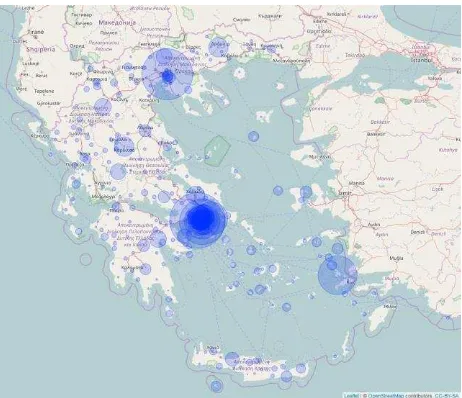
The following R code computes the SAM measure for the 326 administrative areas in Greece (325 Municipalities and the Holly Mountain) to the 132 Hospitals in Greece and plots it using scalable circles (Figure 1).

library(SpatialAcc)

D <- distance(p.coords, h.coords)

SAM.d2 <- ac(p, n, D, d0, power=2, family="SAM")

Results <-

data.frame(PWC.Municipalities[,c(1,5,6)], p, SAM.d2)

library(leaflet)

m= leaflet(Results) %>% addTiles() %>% setView(23, 39, zoom = 6) %>%

addCircles(lng= ~Lon, lat= ~Lat, weight= 1, radius = ~sqrt(SAM.d2) * 200000000, popup = ~KallCode)

m

It is apparent from Figure 1, that Athens and Thessaloniki Metropolitan areas exhibit high accessibility to public hospitals while most of the rest of the country does not. The high SAM value in Kos is due to the large psychiatric hospital in the nearby island of Leros.

Figure 1. Spatial Accessibility to public hospitals

We then compute the Gini coefficient. Since there is no optimal number of nearest neighbours, we try six different numbers and report the results (Table 1). The code below allows for the calculation of the global Gini, its spatial components and their statistical significance using the R-package lctools.

library(lctools)

bw <- c(4, 5, 6, 9, 12, 20)

Gini <- matrix(data=NA, nrow=6, ncol=8)

colnames(Gini) <- c("ID", "k", "Gini", "Gini of neigh.",

"Gini of non-neigh.",

(3)

gini <- spGini(p.coords,b,Results$SAM.d2)

gini.Sim99 <- mc.spGini(Nsim= 99, b, Results$SAM.d2, p.coords$pwX, p.coords$pwY)

Gini[counter,1] <- counter

Gini[counter,2] <- b

Gini[counter,3] <- gini[[1]]

Gini[counter,6] <- 100*gini[[4]]

Gini[counter,7] <- 100*gini[[5]]

Gini[counter,8] <- gini.Sim99[[3]]

counter<-counter+1 coefficient while the third and fourth columns show the Gini of the neighbour and the Gini of the non-neighbour municipalities, respectively. The fifth and sixth columns show what proportion (%) of the overall Gini is the Gini of the neighbour and the Gini of the non-neighbour municipalities, respectively. Finally, the last column shows the p-value which is the result of a Monte Carlos simulation with 99 iterations. If the p-value is lower or equal to 0.05 then we can argue that the spatial components of the Gini coefficient are statistically significant at the 95% level of significance.

Table 1. Sensitivity analysis of the Gini coefficient for SAM

k Gini Gini of inequalities in the spatial accessibility to public hospitals in Greece among municipalities. The Gini of the neighbour areas accounts between 0.8% and 5.6% of the overall Gini for a list of different numbers of nearest neighbours (4, 5, 6, 9, 12 and 20). This suggests a very strong positive spatial autocorrelation in the SAM for the Municipalities in Greece. Indeed, most of the inequality is due to differences in SAM between non-neighbour municipalities. These findings are statistically significant in most cases.

The next step is to look how spatial accessibility varies across certain population groups with different demographic and socioeconomic characteristics. The simplest way to check for

this is by computing the distance to the nearest hospital for each population subgroup. Figures 2-4 present cumulative proportions of population by distance to the nearest hospital. The population has been disaggregated by age, socioeconomic characteristics and educational attainment.

The R code below computes the Euclidian distance to the nearest hospital from the population weighted centroid of each municipality.

PopByAge <- read.csv("PopByAge.csv", sep=";", dec=",")

PopByEconEdu <- read.csv("PopByEconEdu.csv", sep=";", dec=",")

PWC.Municipalities$CodeN <-

as.numeric(PWC.Municipalities$KallCode)

MbyAge <- merge(PWC.Municipalities, PopByAge, by.x = "CodeN",

by.y = "area_code")

MbySocEco <- merge(PWC.Municipalities,

PopByEconEdu, by.x = "CodeN", by.y = "AreaCode")

pbyage.coords <- MbyAge[,3:4] pbysoc.coords <- MbySocEco[,3:4]

D.age<-distance(pbyage.coords, h.coords)/1000 D.soc<-distance(pbysoc.coords, h.coords)/1000

MbyAge$Min.Dist.Hosp <- apply(D.age, 1, min) MbySocEco$Min.Dist.Hosp <- apply(D.soc, 1, min)

Due to several missing values in the demographic and socioeconomic characteristics, the spatial accessibility statistics have been computed for 321 municipalities in the case of age groups and 316 municipalities in the case of socioeconomic groups.

The R code below provides an example on how the above findings can be summarised and plotted using the R package ggplot2. This example results in Figure 2.

breaks= c(0,5,10,15,20,25, 30, 35, 50, 100, 130)

distance = MbyAge$Min.Dist.Hosp distance.cut = cut(distance, breaks)

MbyAge <- cbind(MbyAge,distance.cut) df <- data.frame(dist=breaks[2:11])

for(var in MbyAge[,9:12]) {

xt <- as.data.frame(xtabs(var~distance.cut, MbyAge))

df <- data.frame(df, cum_pc=cumsum(round( 100*xt$Freq/sum(xt$Freq),3))) }

names(df) = c("Distance", names(MbyAge)[9:12])

df.m <- melt(df, id="Distance")

library(ggplot2)

ggplot(df.m, aes(x= Distance, y= value, colour= variable)) +

geom_line(size = 1) + geom_point(size = 1) +

xlab("Distance to nearest hospital (Km)") + ylab("Cumulative % of Population")

It is apparent from Figure 2 that children aged 0 – 14 years old and the working age population (aged 15 – 64 years old) reside

(4)

closer to hospitals compared to older people, especially the very old aged 85 years old and over. This is confirmed also in the analysis by economic activity where the retired live longer distance to the nearest hospital compared to the students and the unemployed. Please note that most unemployed persons in Greece are young people (Figure 3).

Figure 2. Spatial accessibility to hospitals for age groups

Figure 3. Spatial accessibility to hospitals for socioeconomic groups

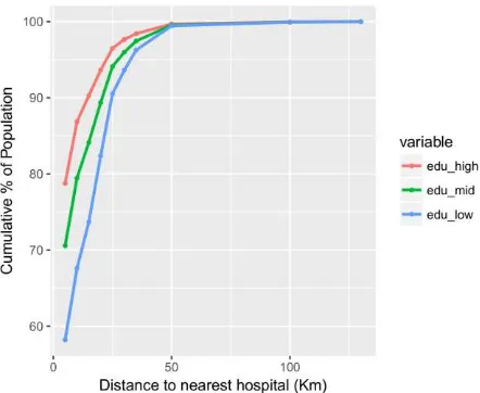
Figure 4. Spatial accessibility to hospitals for groups by educational attainment

It is very clear from Figure 4 that the highly educated are closer to public hospitals compared to those with average educational attainment. People with low educational attainment reside the furthest away from the hospitals compared to the other groups in the category. The findings are similar when road network distance and time are considered instead of Euclidian distance (Kalogirou, 2017b).

4. CONCLUTIONS

The analysis presented in this paper showed inequalities in spatial accessibility to public health services among geographical areas as well as among the population disaggregated by age and socioeconomic characteristics. Certainly, the current locations of public hospitals do not reflect the demographic structure of the country and are far away from the locations older people reside and those most tourists visit. There are serious policy-making implications, especially if we consider that Greece has a population that is rapidly ageing and the country welcomes about 25-30 million tourists every year. We hope that our work will motivate further research on this topic.

REFERENCES

Kalogirou, S., and Foley, R., 2006. Health, Place & Hanly: Modelling Accessibility to Hospitals in Ireland.

Irish Geography, 39(1), pp. 52-68.

Kalogirou, S., and Mostratos, N., 2004. Geographical Access to Health: modelling population access to Greek

public hospitals. In: Proceedings of the 7th Pan-Hellenic

Geographical Congress, Mytilene, Vol.II., pp. 431-437.

Santana, P., 2000. Ageing in Portugal: regional iniquities

in health and health care. Social Science & Medicine, 50,

pp. 1025-1036.

Christie, S., and Fone, D., 2003, Equity of access to

tertiary hospitals in Wales: a travel time analysis. Journal

of Public Health Medicine, 25(4), pp. 344-350.

Kalogirou, S., 2017a. SpatialAcc: Spatial Accessibility Measures. https://CRAN.R-project.org/package=SpatialAcc

Kalogirou, S., 2017b. Spatial analysis of accessibility to public hospitals using GIS, In: Medical Geographical Information: Applications, Analysis and Mapping, SPRINGER, under publication).

Neutens, T., 2015. Accessibility, equity and health care: review and research directions for transport geographers. Journal of Transport Geography, 43, pp 14-27.

Rey, S.J., and Smith, R.J., 2013. A spatial decomposition of the Gini coefficient. Letters in Spatial and Resource Sciences, 6(2), pp. 55-70.