THIN ICE AREA EXTRACTION IN THE SEA OF OKHOTSK
FROM GCOM-W1/AMSR2 DATA
K. Choa, Y. Satoa, K. Naokia
a Tokai University Research & Information Center, 2-28-4, Tomigaya, Shibuyaku, Tokyo, Japan, [email protected] Commission VIII, WG VIII/6
KEY WORDS: Sea Ice, Passive Microwave Radiometer, Ice Thickness
ABSTRACT:
Passive microwave radiometers on-board satellites can penetrate clouds and can monitor the global sea ice distribution on daily basis. The authors have developed an algorithm to extract thin ice area in the Sea of Okhotsk from the passive microwave sensor AMSR2 on-board GCOM-W1 satellite. The algorithm uses the brightness temperature scatter plots of AMSR2 19GHz polarization difference(V–H) vs 19GHz V polarization. The results were verified using simultaneously collected MODIS images in the Sea of Okhotsk. The most of the thin ice areas visually identified in the MODIS images were automatically extracted from AMSR2 data using the algorithm.
1. INTRODUCTION
Sea ice has an important role of reflecting the solar radiation back into space. However, the reduction of ice cover most probably due to the global warming decreases the earth albedo. The decrease of the earth albedo increases the amount of solar energy absorption which accelerates the global warming. This means that the trend of global warming is likely to be enhanced in sea ice areas. Since longer wavelength microwave can penetrate clouds, the passive microwave radiometers on-board satellites, such as SSM/I, ASMR-E and AMSR2, can can monitor the global sea ice distribution on daily basis. The passive microwave radiometer AMSR-E on-board Aqua satellite was launched in May 2002 and operated until October 2011. In May 2012, AMSR2, the successor of AMSR-E, on-board GCOM-W1 was successfully launched by JAXA. On 16 September 2012, the minimum sea ice extent in Northern Hemisphere in the history of passive microwave sensor observation from space since 1978 was recorded by AMSR2 (JAXA, 2012). The importance of sea ice monitoring from space is increasing.
Ice concentration is the most fundamental parameter of sea ice which can be calculated from brightness temperatures measured by passive microwave radiometers. There are number of sea ice concentration algorithms including NASA Team Algorithm (Cavarieli et al., 1984), Bootstrap Algorithm (Comiso, 1995), and ASI Algorithm (Spreen et al., 2008).
Ice thickness is another important parameter of sea ice. Studies on estimating ice thickness from the data acquired from passive microwave radiometers onboard satellites have done in the past including those of Tateyama et al. (2002), Martin et al. (2004, 2005), and Tamura et al.(2007). However, none of them has been adopted as the algorithm for producing sea ice thickness dataset from SSM/I, AMSR-E or AMSR2. This fact reflects the difficulty of estimating ice thickness from passive microwave radiometer.
However, considering the electromagnetic property difference of thin ice against ice floe, the authors think that it is possible to differentiate thin ice area from ice floe. From this perspective, the authors has
been developing methods to detect thin ice
area using brightness temperature acuired from passive
microwave sensor
AMSR-E and AMSR2 (Cho et al., 2012, 2013, Tokutsu et al., 2014). In this paper, the authors willdescrive about the concept of our method and the possibility of using the algorithm for producing thin ice data set of the Sea of Okhotsk from AMSR2 data to be defined as JAXA’s AMSR2 Reserch Product. In thin ice areas, the heat flux of ice is strongly affected by the ice thickness difference (Maykut, 1978). Thus, we believe that this method may contribute to the climate change study. hemisphere. Since the sea ice of the sea are consisted only of first year ice and many thin ice area can be found in the sea, the sea is most suitable test site for developing the thin ice area extraction algorithm.
3. ANALYZED DATA
As for the passive microwave sensor data, the brightness temperature data collected by AMSR2 onboard GCOM-W1 satellite were used. Table 1 show the specifications of AMSR2. In order to identify thin ice area, band 1 and 2 data of the optical sensor MODIS onboard Aqua satellite were also used in this study. Table 2 show the specifications of MODIS. Since Aqua and GCOM-W1 are in the same orbital “track” under the frame work of NASA’s A-Train (2012), MODIS onboard Aqua observes the same area four minutes after the observation of AMSR2 onboard GCOM-W1. This means that we can estimate that the both sensors are observing the same phenomena almost at the same time.
Figure 1. Test Site Sea of Okhotsk The International Archives of the Photogrammetry, Remote Sensing and Spatial Information Sciences, Volume XLI-B8, 2016
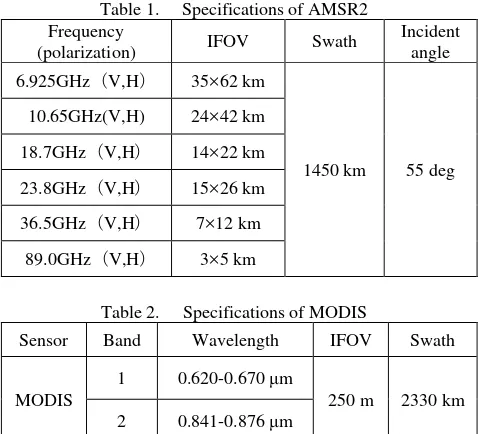
Table 1. Specifications of AMSR2
Table 2. Specifications of MODIS
Sensor Band Wavelength IFOV Swath
MODIS
1 0.620-0.670 µm
250 m 2330 km 2 0.841-0.876 µm
*Only the MODIS bands of IFOV=250m are used in this study.
(a) AMSR2 ice concentration image
(b) MODIS image
Figure 2. Comparison of AMSR2 and MODIS images. (Sea of Okhotsk, February 27, 2013)
Figure 2(a) and (b) show the sea ice concentration(IC) image derived from AMSR2 using Bootstrap Algoritm (Comiso, 1995) and MODIS image taken on February 27, 2013 respectively. In Figure 2(a), black corresponds to IC=0% and white corresponds to IC=100%. Figure 3 shows the schematic diagram of calculating ice concentration (IC) from brightness temperatures derived from passive microwave radiometers. In passive microwave region, due to the emissivity differences, the brightness temperature of big ice floe (TBice: for an example 230K) is much higher than that of open water (TBwater: for an example 130K). Thus, if the brightness temperature TB of certain sea ice area is 180K, we estimate the ice concentration IC of the area with the following equation.
IC= 50% most of the sea ice areas in the image are high. However, if we see the MODIS image of Figure 2(b), we see dark area along the coast of Russia. Most of them are thin ice areas. In other words, if the area is covered with 100% sea ice, we cannot discriminate thin ice area of thin ice.
Basically, the albedo increases as the ice thickness increases. Through the comparison of the in situ ice thickness measurements with data collected by optical sensor on board satellites, the authors have verified that under the less snow cover and cloud free condition, thin sea ice area, where the ice thicknesses are around or less than 20cm, can be identified in MODIS images (Cho et. al., 2012). In this study, the color composite images of MODIS (Band 1 to blue and red, Band 2 to green) were used for identifying sea ice comditions of the test site. In thick ice area, since the albedo of both Band 1 and 2 are high, the area appear in white in the color composite image of MODIS. However, in thin ice area, since the surface and around the thin ice are rather wet, the albedo of Band 2(near infrared) become lower compared with that of Band 1(visible). As a result, most of the thin ice areas appear in purple in the color composite image as sown on Figure 2(b). In this study, we defined these dark purple sea areas in the MODIS images as thin ice areas.
Figure 3. The schematic diagram of calculating ice concentration(IC) from brightness temperature (TB) derived from passive microwave radiometer.
4. TEST AREA EXTRACTION
Figure 4(a)and Figure 4(b) show the comparison of simultaneously collected AMSR2 ice concentration image and MODIS image taken on February 27, 2013. The AMSR2 ice concentrations were derive using AMSR Bootstrap Algorithm (Comiso, 2009). In order to examine the microwave brightness temperature characteristics of big ice floe, thin ice, mixed ice, and open water, the sample area of each item was selected in the MODIS image as shown on Figure 4(a). Then, the sample areas were overlaid on the AMSR2 image and the AMSR2 brightness temperature data of the sample areas were extracted as shown on Figure 4(b). Figure 5 shows the enlarged MODIS image of each sample area.
(a) MODIS image (b) AMSR2 ice concentration Figure 4. Comparison of AMSR2 and MODIS images.
(Sea of Okhotsk, February 27,2013)
(a)Big ice floe (b)Thin ice
(c)Mixed ice (d)Open water Figure 5. Sample area of different ice types extracted from
MODIS image
(Sea of Okhotsk, February 27, 2013)
5. THIN ICE AREA EXTRACTION ALGORITHM In our thin ice area extraction algorithm, we utilize the scatter plots of AMSR2 19GHz polarization difference (V-H) vs 19GHz V polarization. Figure 6 shows the scatter plot of
AMSR2 19GHz V versus 19GHz (V-H) of the Sea of Okhotsk observed on February27, 2013. In this scatter plot, ▲represents thin ice and ■ represents big ice floe. In our thin ice area extraction algorithm, firstly we used the following equation to extract thin sea ice area with 80% or higher sea ice concentration.
(Tb19GHzV) > 245K (2) Tb19GHzV: Brightness temperature of AMSR2 19GHz V
polarization
In low ice concentration sea ice area, since various thickness sea ice and open water are mixed within one footprint area of a passive microwave radiometer, one cannot identify the ice thickness of the area. So, in this study, the thin ice area are only extracted for high ice concentration areas.
Figure 6. Scatter plots of (19GHzV – 19GHzH) Vs 19GHzV polarization (Sea of Okhotsk, February 27, 2013) The microwave brightness temperature of water is much lower in H polarization than in that of V polarization. As explained in chapter 4, thin ice areas are rather wet. Therefore, in thin ice areas, the microwave brightness temperature of thin ice areas become much lower in H polarization than in that of V polarization. While the microwave brightness temperature of consolidated ice does not show big difference between V and H polarization. Considering these characteristics, the authors have introduced the following equation for extracting thin ice area from AMSR2 data.
(Tb19GHzV-Tb19GHzH) > -Tb19GHzV + 300K (3) Tb19GHzH: Brightness temperature of AMSR2 19GHzH
polarization
Since the brightness temperature difference between V and H polarization is much bigger for thin ice than for consolidated ice, extraction of thin ice area can be expected with equation (2) and (3).
6. EXTRACTED RESULT
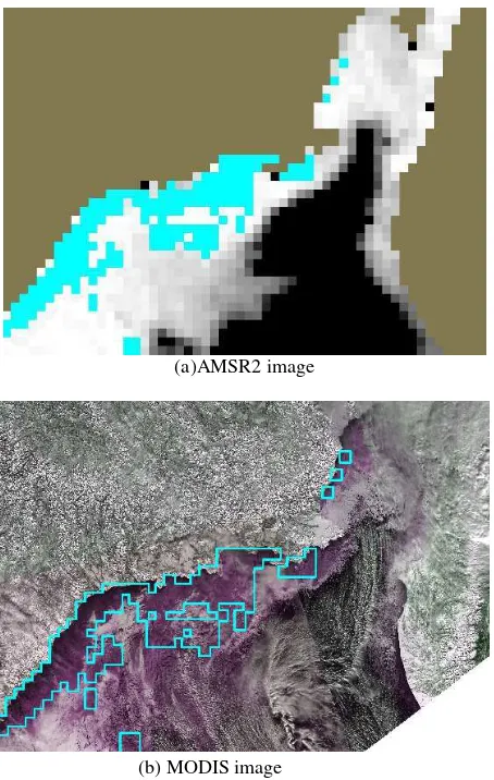
The authors have applied the thin ice area extraction algorithm to AMSR2 data of the Sea of Okhotsk. Figure 7(a) shows the AMSR2 sea ice concentration image of February 27, 2013. The cyan areas in the image show the “thin ice areas” extracted using AMSR2 data using equations (2)and (3). The extracted areas were overlaid on the simultaneously collected MODIS image for evaluation as shown on Figure 7(b). It shows that not all but most of the thin ice areas which are appearing in dark purple in the MODIS image are extracted with this method.
(a) AMSR2 image
(b) MODIS image
Figure 7. Thin ice area extraction result (Cyan: extracted area) (Sea of Okhotsk, February 27, 2013)
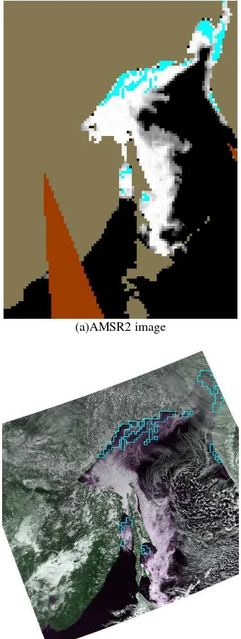
In order to verify the stability of the algorithm the same equations are applied to AMSR2 data of February 7, 15, 23, 26 and March 11, 2014. The brightness temperature data of various sea ice types are plotted on the scatter plots of AMSR2 19GHz V versus 19GHz (V-H) for the Sea of Okhotsk observed on February26, 2014 as shown on Figure 8. Figure 9 show the result of thin ice area extraction. Again, most of the thin ice areas were well extracted in the AMSR2 image. Figure 10 and Figure 11 show the result for February 23, 2014 and Figure 12 and Figure 13 show the result for March 11, 2014.
Figure 8. Scatter plots of (19GHzV – 19GHzH) Vs 19G H polarization (Sea of Okhotsk, February 26, 2014)
(a)AMSR2 image
(b) MODIS image
Figure 9. Thin ice area extraction result (Cyan: extracted area) (Sea of Okhotsk, February 26, 2014)
Figure 10. Scatter plots of (19GHzV – 19GHzH) Vs 19G H polarization (Sea of Okhotsk, February 23, 2014)
(a)AMSR2 image
(b) MODIS image
Figure 11. Thin ice area extraction result (Cyan: extracted area) (Sea of Okhotsk, February 23, 2014)
Figure 12. Scatter plots of (19GHzV – 19GHzH) Vs 19G H polarization (Sea of Okhotsk, March 11, 2014)
(a)AMSR2 image
(b) MODIS image
Figure 13. Thin ice area extraction result (Cyan: extracted area) (Sea of Okhotsk, March 11, 2014)
8. CONCLUSIONS
In this study, authors have developed an algorithm to extract thin ice area using brightness temperature scatter plots of AMSR2 19GHz polarization difference (V-H) vs 19GHz V polarization. The extracted thin sea ice areas were validated by comparing with simultaneously observed MODIS images. The most of the thin ice areas identified in MODIS images were automatically extracted with this algorithm. The authors have processed total of 6 scenes for the Sea of Okhotsk with this algorithm. The result suggested the effectiveness of the algorithm. This new algorithm is now considered as the algorithm for producing the Thin Ice dataset for the Sea of Okhotsk as one of GCOM-W Research Products. Since the heat flux of ice is strongly affected by the ice thickness differences, this product may contribute to the imporvement of the heat flux calculation over the sea ice area.
However, it should be noted that the thin ice areas were extracted only for the areas where the sea ice concentration were higher than around 80% in this algorithm. Also, the definition of “thin ice” in this study is the thin ice areas which can be identified in MODIS images by image interpretation. Josefino Comiso of NASA for his kind advices on our study.
REFERENCES
JAXA, 2012, A new record minimum of the Arctic sea ice xtent, http://www.satnavi.jaxa.jp/project/gcom_w1/news/2012/120920 Bootstrap Algorithm”, NASA Reference Publication 1380, Maryland, NASA Center for AeroSpace Information.
Spreen G., L. Kaleschke, and G. Heygster, 2008, Sea ice remote sensing using AMSR-E 89 GHz channels, J. Geophys. Res., Vol. 113, C02S03, doi:10.1029/2005JC003384.
Tateyama K., H. Enomoto,, T. Toyota. and S. Uto, 2002, Sea ice thickness estimated from passive microwave radiometers, Polar Meteorol. Glaciol., National Institute of Polar Research, Vol. 16, pp.15-31.
Martin S. and R. Drucker, 2004, Estimation of the thin ice thickness and heat flux for the Chukchi Sea Alaskan coast polynya from Special Sensor Microwave/Imager data, 1990–
2001, JGR, Vol. 109, C10012, pp.1-15
Martin S. and R. Drucker, 2005, Improvements in the estimates of ice thickness and production in the Chukchi Sea polynyas
derived from AMSR-E, GRL, Vol. 32, L05505
Tamura T., K. I. Ohshima, T. Markus, D. J. Cavalieri, S. Nihashi, N. Hirasawa, 2007, Estimation of Thin Ice Thickness and Detection of Fast Ice from SSM/I Data in the Antarctic Ocean, Journal of Atmospheric and Oceanic Technology, Vol. 24, pp.1757-1772.
Cho, K., Y. Mochizuki, Y. Yoshida, 2012, Thin ice area extraction using AMSR-E data in the Sea of Okhotsk,
Proceedings of the 33rd Asian Conference on Remote Sensing,
TS-E6-3, pp.1-6.
Cho K., Y. Mochizuki, Y. Yoshida, T. Tezuka, 2013, Thin Ice Area Extraction using AMSR2 Data in the Sea of Okhotsk, Proc. of the International Symposium on Remote Sensing(ISRS) 2013, C7-01, pp.1-4.
Tokutsu Y., K. Cho, 2014, Thin Ice Area Extraction Algorithm Using AMSR2 Data for the Sea of Okhotsk, Proceedings of the 35th Asian Conferenceon Remote Sensing,OS-101, pp.1-6.
Maykut, G. A., 1978, Energy exchange over young sea ice in the central arctic, JGR, Vol.83, pp.3646-3658.
NASA, 2012, Afternoon Constellation, http://atrain.nasa.gov/ Cho K., Y. Mochizuki, Y. Yoshida, H. Shimoda and C. F. CHEN, 2012, A study on extracting thin sea ice area from space, International Archives of the Photogrammetry, Remote Sensing
and Spatial Information Sciences, Vol. XXXIX-B8,
pp.561-566.
Comiso, J. C., 2009, Enhanced Sea Ice Concentrations and Ice Extent from AMSR-E Data, Journal of the Remote Sensing Society of Japan, Vol.29, No.1, pp.199-215.