CHANGES IN SCATTERED GREENERY IN SELECTED AREA IN THE CZECH
REPUBLIC FROM 1953 TO 2014
V.Ždímal a
a Mendel University in Brno, Zemědělská 1, 613 00 Brno, Czech Republic - [email protected]
Commission VIII, WG VIII/8
KEY WORDS: Land Cover, Greenery, History, Distance Analysis
ABSTRACT:
The Land Cover of the Czech landscape could change several times. Reconstructing Land Cover and especially greenery in the past is important for today’s use of the landscape. Two periods were chosen to track changes in scattered greenery, the years 1953 and 2014. The source of information was an historical orthophotomap supplemented with a Military Topographic Map and an orthophotomap supplemented by terrain mapping. The software ArcMap and GuidosToolbox were used. The greenery was highlighted and manually converted to a vector format.
The total area of the monitored territory is 2,190 hectares. In 1953, greenery took up 102 ha and 90 individual green areas were identified here. In 2014, greenery took up 222 ha and it was divided into 113 individual areas. In 1953 the perimeter of all green areas was 41,537 meters; in 2014 the perimeter of all green areas was 89,974 meters. There are two apparent trends here. The first is the simplification of shapes as a result of large-scale management; the second is the formation of a large length of linear greenery and small width with a large perimeter.
The shape of the surface is linked to the area and perimeter. In 1953 this parameter was on average 1.87, and in 2014 the average value was 2.58. Comparing the results of the distance analysis of Label Objects using the GuidosToolbox software found that virtually all green areas were classified differently in 1953 and 2014. The results are completely different and further analysis makes no sense.
1. INTRODUCTION
Czech landscape belongs to old development areas settled by a man from old ages. The landscape has been under human influence since people first arrived on the scene, with individual eras leaving their mark in the form of layers which may be read almost like a palimpsest. A single location may show evidence of human activity from the different periods and natural changes. The Land Cover of one location could change several times. The most important reason is meandering and following straightening of rivers, deforestation and soil movement. In the past those changes influenced today's management and it is important to identify them. When we design a new Land Use is important to know the Land Cover in the past. Knowledge of the Land Cover in the past allows us to propose the appropriate the Land Use in the present and prevent unsuitable use of landscape with limited usage. One of the tools used to determine the different places are archival materials.
Lipský (1999) and Kubeš (1996) describe detailed origin and development of cultural landscape in the Czech Republic. Czech landscape underwent a fundamental change in the period of socialist collectivization of agricultural production since 1954. The area of agricultural land increased, meadows and grassland were arable in the lower altitudes. Usage of plant protection chemicals and chemical fertilizers negatively affected the biota of agricultural land, neighborhood land and biota water streams and reservoirs. Insecticides kill many insects, heavy metals get worse health status and reproductive abilities of birds and mammals, plant species sensitive to nitrogen disappeared and plants able to live in the new conditions appeared. Increasing the area of agricultural land and the change of
management of the meadows and pastures have deteriorated aesthetic parameters of the countryside. In some areas there are occurred increasing of the size of area of woody vegetation of agricultural landscape in the period of socialist collectivization of agriculture. That development was different in each territory of the republic, depending on whether it was a production area or marginal. Large-scale socialist farming practices in the country left a number of small unusable areas with weeds and trees. The current state of the landscape is not very different from the condition of the landscape during periods of maximum application of forms of socialist agriculture.
The Czech Republic has a considerable amount of documentation, which makes it possible to reconstruct the former state of the landscape. The main documents are topographical maps (Skokanová & Havlíček, 2010), cadastres, archival aerial photographs and direct or indirect signs. Most of the documents are only listed here. We can use: the First the Cadaster of Land (1927), the Cadaster of Real Estates of the Czech Republic (1993), the aerial photographs (1938-2014), and more.
Topographical maps and cadastres depict the landscape relatively well, but only at some point. A long period of time The International Archives of the Photogrammetry, Remote Sensing and Spatial Information Sciences, Volume XLI-B8, 2016
still needs to be depicted. And the consequences of the activity of these unknown periods need not have an effect on anything smaller. Identifying them is possible with field research and observations made from above on the basis of direct or indirect signs.
Historical orthophotomap from the year 1953 is the most important material for the study of historical Land Cover of the Czech Republic. For purposes of creation of this orthophotomap aerial photographs and reconnaissance photographs from the aerial photographs archive of the Czech Republic (managed by Military Geographic and Hydrometeorlogic Office - MGHO) were used. When selecting suitable aerial photographs from the post-war period, the date of acquisition as close as possible before the time of collectivization during the years 1952 and 1953 was primarily respected. Verification of archives of aerial photographs proved that photography in the years after World War II was relatively fragmented and cover of the entire territory of the Czech Republic was attained between 1946 and 1959. Some places were not covered by the post-war images at all (before the collectivization). These places were covered with aerial photos from pre-war period and images taken in 1959. selected area is among the localities with less representative greenery, since the forest cover in the Czech Republic is approximately 33%.
In the area of interest from 1953 to 2003, there were significant changes between different categories of the Land Use. Area of the arable land decreased from 83% to 73%, area of permanent grassland decreased from 7% to 2% and area of the forest land increased from 5% to 10%. The categories of orchards and gardens area occurred increasing by 7% and other categories by 6%. The increase in the category of the others was mainly due to increase in built-up area.
2.2 Data processing
Two periods were chosen to track changes in scattered greenery, the years 1953 and 2014. The source of information was an historical orthophotomap supplemented with a Military Topographic Map from 1953, and 2014 was represented by an orthophotomap from this period supplemented by terrain mapping (Skokanová & Havlíček, 2010, Pelantová, 1994).
Figure 1. Study site
The first step was to use a Histogram Equalization to highlight the greenery in the GuidosToolbox software. GuidosToolbox is Graphical User Interface for the Description of image Objects and their Shapes and contains a wide variety of generic raster image processing routines, including related free software such as GDAL (to process geospatial data and to export them as raster image overlays in Google Earth), and FWTools (pre/post-process and visualize any raster or vector data). (Voght, 2014) The result are shown in Figures 2 and 3. Subsequently, the greenery was manually converted to a vector format in the ArcMap geographic information system. The map was used to check the results for 1953 (the Military Topographic Map, 1953), terrain mapping for 2014. Terrain mapping was also used to validate the data obtained.
The study involves planar and linear greenery. In classifying according to individual categories, the priority was feature, not shape. But in this work, planar and linear greenery were combined into one category.
Figure 2. Original ortophotomap from 1953 The International Archives of the Photogrammetry, Remote Sensing and Spatial Information Sciences, Volume XLI-B8, 2016
Figure 3. The result of Histogram Equalization
The vector data of polygon categories made it possible to measure the total expanse of greenery, the expanse of individual green areas, the perimeter of individual green areas, and the shape of the areas using the Formula 1 in both periods.
�� =2√��� (1)
where Di = shape of the area
P = perimeter of individual area A = area
in both periods. The shape of the area is one in the case of a circle. It also allowed a comparison between the two periods and an overall change in the area and place where the greenery has shrunk or expanded.
The GuidosToolbox software was used to further analyze the distance between patches and the function Label Objects was used. This feature characterizes the relationship between green areas. The software divides the area into several main categories: core, islet, perforation, edge, loop, bridge, branch and background. The output of the software consists of four files containing labeled objects in alternating colors, unique identifiers of the objects, number of pixels for each object and table listing the number of pixels for each object.
3. RESULTS AND DISCUSSION
The conversion to vector format was greatly facilitated by the histogram features, because the highlighted greenery in the GuidosToolbox software facilitated the identification of green spaces, therefore speeding up the manual conversion.
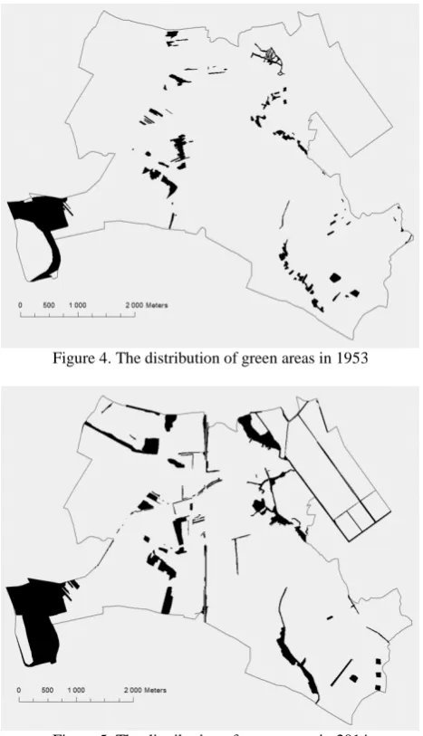
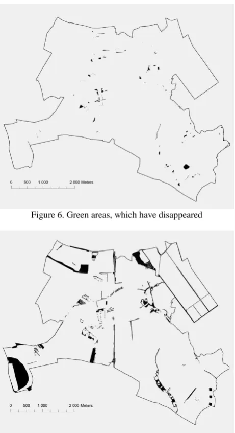
The total area of the monitored territory is 2,190 hectares. In 1953, greenery took up 102 ha, i.e. approximately 5% of the territory and 90 individual green areas were identified here. In 2014, greenery took up 222 ha, i.e. approximately 10% of the territory and it was divided into 113 individual areas. The distribution of green areas in 1953 and 2014 is shown in Figures 4 and 5. A comparison of green areas in 1953 and 2014 allows us to determine which areas have been preserved, which areas have disappeared, and which areas have been added (Figure 6 and 7). The area preserved consists of 91 ha, shrunk areas 12 ha, and added areas 131 ha. This means that a relatively small proportion of greenery has shrunk, but a significant portion of greenery has been added.
Figure 4. The distribution of green areas in 1953
Figure 5. The distribution of green areas in 2014
From the point of view of the landscape, the ecotone parameter is important, i.e. the perimeter of the individual green areas. An ecotone is a transition area between two biomes. An ecotone may appear on the ground as a gradual blending of two communities across a broad area, or it manifest itself as a sharp boundary line. In 1953 the perimeter of all green areas was 41,537 meters; in 2014 the perimeter of all green areas was 89,974 meters. (Table 1) The perimeter of green areas has increased to more than double. There are two apparent trends here. The first is the simplification of shapes as a result of large-scale management; the second is the formation of a large length of linear greenery and small width with a large perimeter. The claim of the authors (Lipský, 1992) cannot be confirmed, as the trend in the monitored area is the opposite.
Variable 1953 2014
Greenery area 102 222
Number of areas 90 113
Perimeter of areas (m) 41,537 89,974
Averaga shape 1.87 2.58
Table 1. The results of the quantitative analysis The International Archives of the Photogrammetry, Remote Sensing and Spatial Information Sciences, Volume XLI-B8, 2016
Figure 6. Green areas, which have disappeared
Figure 7. Green areas, which have been added
The shape of the surface is linked to the area and perimeter. In 1953 this parameter was on average 1.87, and in 2014 the average value was 2.58. Because a circle has a value of 1, and the above trends are in progress, it can be said that from 1953 to 2014 the shape of the areas has been lengthened.
The distance analysis in the software made it possible to monitor spatial patterns and their changes over time. Comparing the results of the distance analysis of Label Objects using the GuidosToolbox software found that virtually all green areas were classified differently in 1953 and 2014. It is the result of a large increase in the area of green spaces from 1953 to 2014, and changes in the shape of the green spaces (Table 2 and Figure 8 and 9). The results are completely different in 1953 and 2014 and further analysis makes no sense.
Land surveying in 2014 was also used to validate the current orthophotomap. Terrain mapping makes it possible to accurately determine the type and elevation of greenery, but in terms of size, shape and location of green areas, the orthophotomap provided an adequate basis.
Class Color
Core
Islet
Perforation
Edge
Loop
Bridge
Branch
Background
Table 2. Resulting class names and colors (Voght, 2007)
Figure 8. The results of the distance analysis of Label Objects using the GuidosToolbox software in 1953
Figure 9. The results of the distance analysis of Label Objects using the GuidosToolbox software in 2014
Reconstructing greenery in the past is important for today’s use of the landscape, because a specific location provides information about the past, e.g. in the form of soil characteristics, and it restricts today’s management.
4. CONCLUSIONS
Historical and current orthophotomaps are suitable for capturing greenery in a given period. Using orthophotomaps makes it The International Archives of the Photogrammetry, Remote Sensing and Spatial Information Sciences, Volume XLI-B8, 2016
Maps, however, enhance orthophotomaps with information on the type of greenery and possibly its height. Conversely, terrain mapping currently makes it possible to validate present-day orthophotomaps. The geographic information system ArcMap and software GuidosToolbox have been suitably for highlight the greenery, convert to a vector format, measure the total expanse of greenery, the expanse of individual green areas, the perimeter of individual green areas, and the shape and the distance analysis. The results are completely different in 1953 and 2014 and further analysis makes no sense. Reconstructing especially greenery in the past is important for today’s use of the landscape, because a specific location provides information about the past and it restricts today’s management.
REFERENCES
Forman, R. T. & Godron, M.1986. Landscape Ecology. John Wiley & Sons, New York, p. 619. ISBN 0-471-87037-4.
Kubeš, J., 1996 Plánování venkovské krajiny. MŽP, Praha, 186 p.
Lipský, Z., 1992 Analýza dlouhodobého vývoje krajiny a její využití pro obnovu ekologické stability. IAE VŠZ, Kostlec n.Č.l. Lipský, Z., 1999 Krajinná ekologie. Karolinum, Praha, 129 p. Pelantová, J. et al, 1994. Metodika mapování krajiny. VaMP - ČÚOP, Praha, 1994, p. 60.
Skokanová H., Havlíček M., 2010. Military Topographic Maps of the Czech Republic from the First Half of the 20th Century. Acta Geod. Geoph. Hung. 45, pp. 120–126.
Šafář, V. et al, V. 2012 Identification of Land Cover in the past using infrared images at present. In: The International Archives of the Photogrammetry, Remote Sensingand Spatial Informatin Sciences, Vol. XXXIX, Part B7, pp. 229-234.
Vogt et al, 2007 Mapping landscape corridors. Ecological Indicatorts, 7, pp. 481-488.
Vogt, P., 2014 GuidosToolbox (Graphical User Interface for the Description of image Objects and their Shapes): Digital image analysis software collection. Available online: <http://forest.jrc.ec.europa.eu/download/software/guidos>. Accessed on: 04.nov.2014