Manajemen | Fakultas Ekonomi Universitas Maritim Raja Ali Haji 073500103288619395

(1)

Full Terms & Conditions of access and use can be found at

http://www.tandfonline.com/action/journalInformation?journalCode=ubes20

Download by: [Universitas Maritim Raja Ali Haji] Date: 13 January 2016, At: 00:20

Journal of Business & Economic Statistics

ISSN: 0735-0015 (Print) 1537-2707 (Online) Journal homepage: http://www.tandfonline.com/loi/ubes20

Semiparametric Duration Models

Feike C Drost & Bas J. M Werker

To cite this article: Feike C Drost & Bas J. M Werker (2004) Semiparametric Duration Models, Journal of Business & Economic Statistics, 22:1, 40-50, DOI: 10.1198/073500103288619395

To link to this article: http://dx.doi.org/10.1198/073500103288619395

View supplementary material

Published online: 01 Jan 2012.

Submit your article to this journal

Article views: 67

View related articles

(2)

Semiparametric Duration Models

Feike C. D

ROST

and Bas J. M. W

ERKER

CentER, Department of Econometrics, and Department of Finance, Tilburg University, P.O. Box 90153, 5000 LE, Tilburg, The Netherlands

In this article we consider semiparametric duration models and efcient estimation of the parameters in a non-iid environment. In contrast to classical time series models where innovations are assumed to be iid we show that in, for example, the often-used autoregressive conditional duration (ACD) model, the assumption of independent innovations is too restrictive to describe nancial durations accurately. There-fore, we consider semiparametric extensions of the standard specication that allow for arbitrary kinds of dependencies between the innovations. The exact nonparametric specication of these dependencies determines the exibility of the semiparametric model. We calculate semiparametric efciency bounds for the ACD parameters, discuss the construction of efcient estimators, and study the efciency loss of the exponential pseudolikelihood procedure. This efciency loss proves to be sizeable in applications. For durations observed on the Paris Bourse for the Alcatel stock in July and August 1996, the proposed semiparametric procedures clearly outperform pseudolikelihood procedures. We analyze these efciency gains using a simulation study conrming that, at least at the Paris Bourse, dependencies among rescaled durations can be exploited.

KEY WORDS: Adaptiveness; Durations; One-step improvement; Semiparametric efciency.

1. INTRODUCTION

Over the last decade, the availability of nancial data at a tick-by-tick level has greatly increased. The irregularly spaced data require new econometric techniques to extract the eco-nomic information contained in such data. This article concen-trates on the durations between transactions on nancial mar-kets. To that extent, we base ourselves on the autoregressive conditionalduration (ACD) model of Engle and Russell (1998). For the data at hand, the traditional assumption of indepen-dently and identically distributed (iid) innovations seems to be inappropriate. Therefore, we need to extend the traditional semiparametric time series models in which innovationsare iid. We consider a sequence of semiparametric models imposing less and less structure on the innovations (with iid innovations on the one end of the specication and martingale innovations on the other end). To obtain efcient estimators in these semi-parametric models, we must extend the semisemi-parametric results available from the emerging literature on semiparametrics.

During recent years, enormous progress has been made in the area of semiparametric estimation. Starting with the work of Stein (1956) on the possibility of adaptiveness in the sym-metric location model, the techniques have been further devel-oped ever since. The work by Hájek (1970) and Le Cam (1986) is especially worth mentioning here. Traditionally, the models considered are based on iid observations. A fairly complete account on the state of the art in iid models can be found in the monograph by Bickel, Klaassen, Ritov, and Wellner (1993). Newey (1990) provided an overview from an econometric per-spective. Semiparametric efciency considerations and adap-tiveness in time series have also been discussed, beginning with Kreiss (1987a, 1987b) for autoregressive moving average-type models. In this stream of literature, the innovationsare assumed to be iid. Koul and Schick (1997) discussed nonlinear autore-gressive location models, with special emphasis on the initial value problem. Drost, Klaassen, and Werker (1997) considered so-called group models, covering nonlinear location-scale time series. Steigerwald (1992) studied linear regression models in a time series context. Linton (1993) discussed linear models with autoregressive conditional hetero-scedasticity (ARCH) errors.

Drost and Klaassen (1997) particularized to the generalized ARCH (GARCH) model, and Wefelmeyer (1996) calculated efciency bounds in models with general Markov-type tran-sitions. In this article we discuss the ACD model, which is, probabilistically, closely related to the ARCH-type models. However, all previous work on semiparametric efcient estima-tion for ARCH-type models assumed the innovaestima-tions to be iid, an assumption that we relax signicantly.

In this article we drop the iid assumption on the innovations. The semiparametric techniques mentioned earhier are used and extended to build an adequate model for durations between transactions on nancial markets. Therefore, we consider semi-parametric specications in which the innovationsmay have de-pendenciesof unknown functionalform. As shown in Section 2, such a specication leads to a nontrivial analysis of semipara-metric efciency. The empirical results in Section 4 show that the gains from considering these more complicated semipara-metric procedures may be important, at least for the present dataset and under the imposed hypotheses. Whether sizeable gains are available in other situations remains an empirical is-sue. Possible efciency gains are important because they allow for much more precise parameter estimates and predictions. Also, in nancial applications, where the number of observa-tions is typically large, this may lead to a more precise empiri-cal analysis.

The crucial ingredient in semiparametric efciency calcula-tions is theefcient score function. Let us recall this concept

here. (For a rigorous treatment, consult, e.g., Bickel et al. 1993 or Drost et al. 1997.) Consider a setup whereidenotes the ob-servation number andµ₂2is a nite-dimensional parameter of interest. Denote (conditional) expectations underµ byEµ.

In general, a score functionsi._¢/is a random function of the parameterµ, such that

Eµ0fsi.µ0/g D0; µ022; iD1; : : : ;n: (1)

(3)

Generally, the expectation in (1) must be conditional on “the past” to get a martingale structure allowing for the deriva-tion of limiting distribuderiva-tional results of estimators based onsi. AZ-estimatorµObased on the score functionsiis subsequently dened as the solution of

1

n

X

i_D1

si.µ /O D0:

In parametric settings, the optimal score function is given by the derivative of the conditional log-likelihood for µ. An es-timator based on the parametric score function is clearly in-feasible in a semiparametric situation. However, the key idea in a semiparametric setting is to reduce the problem to a spe-cic well-chosen parametric one. This special parametric model is called theleast-favorable parametric submodel(cf. Newey 1990). For completeness, we repeat the argument here. First, consider an arbitrary parametric submodel of the semiparamet-ric model under consideration.Obviously, because the informa-tion for statistical inference decreases if one enlarges the model, a lower bound (evaluated at distributions within the paramet-ric submodel) on the asymptotic variance of estimators in the parametric submodel is also a lower bound for the behavior of estimators in the semiparametric model. Because this holds for any parametric submodel, the lower bound on the asymptotic variance of semiparametric estimators must be larger than each of these parametric lower bounds. Thus the supremum of the lower bounds over the class of all parametric submodels also gives a lower bound for the semiparametric model. The particu-lar parametric submodel for which this supremum is attained (if it exists) is called theleast-favorable parametric submodel. The

second problem is to prove that a given lower bound is sharp. Usually, sharpness of a given bound is proved by providing a semiparametric estimator attaining this bound. Hence, if one nds a parametric submodel and an estimator in the semipara-metric model such that the bound of the parasemipara-metric submodel is attained by the semiparametric estimator, then the bound is sharp and the estimator is efcient.

To nd the least-favorable submodel, a technique based on tangent spaces has proved to be very useful (see, e.g., Bickel et al. 1993; Van der Vaart 1998). If one passes from a parametric model (say a model in which the densityf of the innovationsis

completely known) to a semiparametric model where one sup-poses thatf is unknown, then there is usually an efciency loss.

This efciency loss is caused by local changes in the density

f that cannot be distinguished from local changes in the

pa-rameter of interestµ. Let Pldenote the score function forµ in the parametric model. The tangent space forf is dened as the

space generated by all possible score functions for the nuisance parameter, that is, those score functions that can be obtained by changes in the nonparametric nuisance parameter,f. The least-favorable parametric submodel induces a nuisance score (i.e., an element of the tangent space) that is closest to the scorePl

induced by µ. This nuisance element is, by construction, the projection oflPonto the tangent space. The residual of this

pro-jection denes the information left for estimatingµ oncef is

unknown. This residual is called theefcient score function. In

this article we extend this idea to the situation where innova-tions are not likely to be iid (as in duration models). The known procedure for time series models with iid innovationsis adapted

to cover several forms of dependencies.In Section 2 we develop the necessary theory leading to the relevant tangent spaces and efcient score functions of the parameters of interest.

The article is organized as follows. In Section 2 we discuss duration models in their general form and develop the semi-parametric theory as discussed earlier for the non-iid setting at hand. Examples (Sec. 2.3) show how common specica-tions may be obtained. These specicaspecica-tions include different assumptions on the innovations, like iid-ness or a Markov-type assumption. We consider the estimation problem in Section 3. We consider the consistency and efciency of pseudolikelihood procedures and a construction generally leading to efcient semiparametric estimators. These semiparametric procedures prove superior to pseudolikelihood procedures. In Section 4 we discuss the properties of the durations observed on the Paris Bourse for the Alcatel stock in July–August 1996. We choose this sample because it has been considered previously in the literature (see, e.g., Ghysels, Gourieroux, and Jasiak, in press; Gourieroux and Jasiak 2000). To give a possible explanation for the semiparametric efciency gains observed in Section 4, we study some parametric extensions of the basic ACD model in Section 5. These extensions are chosen such that they ex-hibit similar dependencies as we nd in the Alcatel data. The simulation study in Section 5 conrms the empirical ndings of Section 4. Finally, in Section 6 we provide some concluding remarks.

2. THE AUTOREGRESSIVE CONDITIONAL DURATION MODEL

2.1 The Parametric Autoregressive Conditional Duration Model

In this article we focus on the autoregressive conditional du-ration (ACD) model as introduced by Engle and Russell (1998). Suppose that we observe durationsx1; : : : ;xn. Thesex’s repre-sent the time elapsed between two events, for example, transac-tions of some asset. LetF_i_{denote the information available for}

modelingxi_C1;xi_C2; : : :. We setF_i_D_{¾ .}_x_i;_x_i_¡₁_{; : : : ;}_x₀_/_{, but it}

is very well possible to include exogenous variables inF_i_{. This}

is because the derivations that follow are independent of the parametric form of the conditionaldurationÃi_¡1dened in (2).

Such extra exogenous variables would allow other observable factors to inuence the distribution of future durations.

The key ingredient in the ACD model is the (conditional) mean duration time,

E_fxijFi_¡1g DÃi_¡1: (2) In its simplest form, the formulation of the ACD model is com-pleted by stipulating, for example,

P_f_x_i_·_x_jF_i_¡₁_{g D}F.x=Ãi¡1/ (3) and

ÃiD®C¯xiC° Ãi¡1; (4) where F denotes a particular distribution function (or a para-metric set of distribution functions) on the positive half-line. In this case, the parameter of prime interest isµ _D.®; ¯; ° /T. In its original parametric setting, standard choices ofFinclude the

(4)

exponential distribution and, as an extension, the gamma and lognormal or Weibull distributions. The distributionF has to

be normalized to have expectation one to identify the constant in the specication ofÃi. If F is not specied parametrically, we obtain a semiparametric model. The model (3) is implic-itly based on underlying iid innovations.It is not difcult to see that (3) is equivalent to saying that

"iDxi=Ãi¡1 (5)

denes a sequence of iid-positive random variables, each with distribution function F. Moreover, note that the ACD model is closely related to ARCH-type models. Rewriting (5), with ´2_i _D"i,y2i Dxi, and¾i2_¡1DÃi¡1, yieldsyiD¾i¡1´i, the stan-dard ARCH formulation. Our results are thus easily adapted to ARCH-type models. Finally, note that all of our results rely on the assumption that the conditional mean equation is correctly specied, as in other works in the literature.

The foregoing ACD model, including various extensions, was introduced by Engle and Russell (1998) and also studied by Engle (2000) together with a modeling of prices. These au-thors explicitly recognized the fact that the independence as-sumption in (3) implies that all temporal dependence between durations is supposed to be captured by the conditional mean duration functionÃi. In that case, several parametric and non-parametric specications of the distribution of the innovations

Fhave been studied. Zhang, Russell, and Tsay (2001) relaxed

the independence assumption on the innovations by introduc-ing a parametric regime-switchintroduc-ing model. In this article we re-lax the assumption of independent innovationsto semiparamet-ric alternatives. We specify the general model in the next sec-tion.

2.2 The Semiparametric ACD Model

Often, the strong iid assumption (3) is considered to be un-suitable and one would like to relax it. In our specication, this is equivalent to allowingFto be dependent on the past as well. If it is unknown in what way F should depend on the past, a semiparametric approach seems to be the most reasonable one. We assume that one is willing to dene a set of variables that may inuenceF, and we see that the actual choice of these variables inuences the semiparametric analysis. In complete generality, we assume thatP_f"i·"jFi¡1gisHi¡1measurable,

whereH_i_¡₁_½F_i_¡₁_{. So the restricted information set}H_i_¡₁_(of

the full information setF_i_¡₁_{) denes the relevant past variables}

to be used as parameters in the conditional distribution of the innovations"i. As we show, the situation whereHi¡1is strictly

smaller thanF_i_¡₁is both common and relevant. We do not

as-sume that.H_i/forms a ltration; that is,H_i_¡₁is not necessarily

included in H_i. This allows for, for example, semiparametric

Markov models, see below.

Formally, our semiparametric model is now described by (2) and

L .xi=Ãi¡1jF_i_¡₁/_DL .xi=Ãi¡1jH_i_¡₁/; a.s. (6) One may choose the specication (4) of Ãi, but other choices (like the ones in Engle 2000) do not change the arguments pre-sented later. Writing "i Dxi=Ãi¡1, we clearly have from (2)

that E_f"ijFi¡1g D1. We do not make other assumptions on

the innovation’s distribution, although later some assumptions are needed for the nonparametric estimation. It is known that symmetry of the density sometimes helps in semiparametric estimation. In the present case, given the positiveness of du-ration, symmetry could be imposed for the distribution of the log-innovations.We do not make such an assumption, because its empirical foundation is unclear at the moment. Note that in our specication (6), the choice of the restricted information set

H_iformalizes the dependence among the innovations"i. A model with independent innovations can be obtained by takingH_i_{equal to the trivial sigma eld, that is,}H_i_{D f}?_{; Ä}_g. There are two other important cases. By choosingH_i _DF_i_,

one leaves the dependence structure of the"i completely un-restricted. In more familiar terms, this would lead to a model characterized solely by the moment condition (2). One could also set H_i_D_{¾ ."i/}_{. In that case, the conditional distribution}

of"i, given the past, may only depend on "i¡1. This induces

a rst-order Markov assumption on the innovations. In a sim-ilar manner, one can study the effect of aK-order Markov

as-sumption by takingH_i_D¾ ."i; : : : ; "iC1_¡K/. Of course, there are many more possibilities. The theoretical derivations in the rest of this article are based on a general specication with an arbitrary choice ofH_i_{, and we specialize to the aforementioned}

choices to point out their differences from an estimation stand-point in Section 2.3.

To derive efciency bounds in the semiparametric model de-scribed by (2) and (6) with an arbitrary specication of the con-ditional expected durationÃi¡1andHi¡1, we follow the steps

as set out in Section 1. Letµ denote the Euclidean parameter of interest describing the functional form of the conditional mean durationÃi_¡1, for exampleµ_D.®; ¯; ° /T in (4). Writefi_¡1for

the density associated withL ."ijHi¡1/. We assume thatfi¡1

ad-mits a Radon–Nikodym derivativef_i0_¡₁, i.e.,fi¡1can be written

as

fi¡1."/_D

Z "

0

f_i0_¡₁.u/du:

Note that this rules out, for instance, a uniform innovation dis-tribution. Regularity conditions under which the results pre-sented later hold are standard in the semiparametric literature (see, e.g., Bickel et al. 1993, sec. 2.1; Drost et al. 1997, sec. 2). The score function forµcan be obtained by differentiationof the log-likelihood,

P

li.µ /_D d

dµ log

³ ₁

Ãi_¡1fi¡1.xi=Ãi¡1/

´

D ¡

³

1_C"i

f_i0_¡₁."i/

fi_¡1."i/

´

d

dµ log.Ãi¡1/: (7) To obtain the efcient score function in the semiparametric model in which the conditional densityfi_¡1 remains

unspeci-ed, we need to calculate the projection of the scorePli.µ /on the tangent space generated by the nuisance functionfi_¡1. As

we argue along the general lines of, for example, Bickel et al. (1993), this tangent spaceTi.µ /is generated by all observation

iscore functionshi¡1._¢/for which

hi_¡1._¢/₂H_i_¡₁_; ₍₈₎

0_DE_fhi¡1."i/jHi¡1g D

Z

"

hi¡1."/dP_f_"_i_·_"_jH_i_¡₁_g; (9)

(5)

and

0_DE_f"ihi¡1."i/jHi¡1g D

Z

"

"hi¡1."/dP_f"i·"jHi¡1g: (10) Because we have only two conditions onfi, we have two con-ditions on the scores in the tangent space. Condition (8) fol-lows from the fact thatfi_¡1is known to depend onHi_¡1only,

so that scores obtained by local changes in fi¡1 also depend

on H_i_¡₁ only. Condition (9) is the standard constraint in

tan-gent space calculations, following from the fact that densi-ties by denition integrate to 1. In more classical terms, this represents the condition that expectations of score functions are always 0 [cf. (1)]. Finally, condition (10) results from the moment restriction E_f"ijHi¡1g DE_f"ijFi¡1g D1. The

argu-ment is as follows. Local changes in fi¡1 represented by the

score hi¡1 induce a change in the rst (conditional) moment

of R

""hi¡1."/dPf"i·"jHi¡1g. However, this moment is

re-stricted to be 1 by condition (2). Therefore, the change must always be 0—otherwise, one would not remain in the specied model. With these ingredients, we are ready to state the key proposition providing the lower bound for estimation of the pa-rameters inÃi of the general semiparametric model described by (2) and (6).

Proposition 1. In the semiparametric model described by (2) and (6), the projection of the score functionPli.µ /in (7) on the

Proof. First, note that the proposed projection (11) indeed belongs to the tangent space Ti.µ / because it satises condi-tions (8)–(10). Second, the residual of the proposed projection ofPli.µ /can be written as

We show that both terms on the right side are orthogonal to the tangent spaceTi.µ /. Lethi_¡12Ti.µ /be arbitrary. Then for the

From (9) and (10), we see that the latter term equals 0, proving the desired orthogonality.

For the second term in (12), we obtain

E

where the last equality follows from (6). It is easily seen that this expression equals 0, by rst conditioning on H_i_¡₁_{. This}

completes the proof.

The proof of the foregoing proposition is indirect. Only very few constructive arguments for obtaining efcient score func-tions are known in the semiparametric literature. It is impor-tant to note that the efcient score functions is, as a projection, unique (see, Newey 1990 for a more general discussion).

As mentioned before, the residual (12) of the projection (11) is the efcient score function, which we denote bylP_i¤.µ /. Op-timal semiparametric estimators must be based on this score function. However, (12) cannot be used directly, because it de-pends on the unknown densityfi_¡1and onE_f.d=dµ /log.Ãi_¡1/_j

H_i_¡₁_g. In Section 3.2 we discuss how to estimate fi¡1 and E_f.d=dµ /log.Ãi¡1/_jH_i_¡₁_gto get a semiparametrically efcient

estimator ofµ.

Adaptiveness occurs (by denition) in the case where the efcient score function (12) equals the parametric score func-tion (7). Thus adaptiveness means that the projecfunc-tion of the parametric score on the tangent space is 0. In that case, there is (asymptotically) as much information in the semiparamet-ric model as in the parametsemiparamet-ric model for estimating µ; the parametric score and the semiparametrically efcient score coincide. In the ACD model (4), we have Ãi¡1>0.

There-It is easily seen that for some positiveci_¡1, this is equivalent to

fi¡1."/_D c

(6)

Hence adaptiveness occurs if and only if the conditional in-novation’s distribution is of the gamma type (rescaled to have expectation 1). Note that the free parameterci¡1may be

time-varying and thus that innovations need not be iid for adaptive-ness to occur. A similar result has been obtained for location models where adaptiveness occurs for the normal distribution and symmetrized square roots of chi-squared distributions (see González-Rivera 1997). In our scale case, we have adaptive-ness for the exponential and gamma distributions. The practical consequence of such a result is, of course, limited, because the bound is calculated in a model that does not make any distribu-tional assumptions.

It is well known that densities at which adaptiveness occurs also are often the densities for which the pseudo–maximum likelihood estimator (PMLE) is consistent (see, e.g., Bickel 1982). This shows that a PMLE-type estimator is consistent if and only if it is based on a gamma distribution. Because for these densities 1_C"f0."/=f."/is always proportional to 1_¡", the PMLE estimators obtained are in fact identical, and the re-sulting PMLE is based purely on the moment condition (2). The estimator thus obtained is consistent in the full semiparamet-ric model. In Section 3.1 we explain that the PMLE is only semiparametrically efcient under very restrictive conditions. We give an alternative estimator that is semiparametrically ef-cient in the model under consideration in Section 3.2.

The information for estimatingµ in the parametric model is given by the variance of the parametric score (7). Assuming stationarity, this yields

whereJf denotes the Fisher information for scale, that is,

Jf D

The information loss of the semiparametric model, with respect to the parametric model, is given by the variance of (11),

E

Note that the information loss is indeed 0 (adaptiveness) if and only if the (conditional) density fi¡1 belongs to the gamma

class. This follows, because we have, by the Cauchy–Schwarz inequality,

mation in the semiparametric model is given by the variance of

the residual of the projection that, by the Pythagorean theorem, equals

We consider the efciency calculationsin more detail in three specic models.

Example 1(IID Innovations). In the case where the restricted

information set H_i is the trivial sigma-eld, we obtain that

P

Ã _DE_f_dd_µlog.Ãi¡1/_jH_i_¡₁_g is a vector of constants. This

im-plies that all components of the projection (11) generate the same direction in the tangent space Ti.µ /. Moreover, in this case,fi¡1Df. Adaptiveness in such models is well studied (see

Drost et al. 1997). The efcient score function becomes

P

Example 2(Markov Innovations). In a true Markov setting

of the innovations, one would takeH_i_D¾ ."i/. The efcient score (12) does not simplify in this Markov case,

P

General statements are difcult to make in this setting. Clearly, the rst-order Markov case is easily generalized to higher-order Markov settings.

Example 3(Martingale Condition). Consider the case where

H_i _DF_i_{. In that case, the second factor in (11) reduces to} In this expression, the (conditional) density fi¡1 enters only

through var_f"ijHi¡1g. This shows that the semiparametrically

efcient estimator ofµ is the moment estimator based on (2) with (optimal) instrument

1 var_f"ijHi¡1g

d

dµ log.Ãi¡1/:

Note that our general semiparametric approach shows that in the present example, the optimal semiparametric estimator is a moment estimator. We did not limit attention to moment es-timators a priori. Wefelmeyer (1996) obtained similar results in more general models specied in terms of conditional mo-ments conditions only. Note that the same efcient score would

(7)

be obtained in any model whereH_i_¡₁containsdlogÃi¡1=dµ, that is,H_i_¡₁_¾¾ .dlogÃi¡1=dµ /. The efcient score does not change if one enlarges such a model to the martingale model withH_i_DF_i. One may also turn this argument around. Starting

from a model that is solely characterized by the relation (2), no statistical information is added if one imposes the conditionthat the conditional distribution of the innovations given the past

F_i_¡₁_{is determined by}dlogÃi¡1=dµ alone. In that sense,

adap-tiveness occurs between these two situations. However, the con-struction of efcient estimators is much simpler in cases where the restricted information setH_i_¡₁_{is not too large. Therefore,}

from a practical standpoint, alternative specications of the re-stricted information set H_i_¡₁_{, like the one that we use in}

Sec-tion 4, are relevant.

3. ESTIMATION IN SEMIPARAMETRIC AUTOREGRESSIVE CONDITIONAL

DURATION MODELS

3.1 Pseudolikelihood Procedures

The most basic ACD models assume that innovations are iid and exponentially distributed. This assumption has been easily rejected in several studies (see, e.g., Engle and Russell 1998; Engle 2000), but it can be used in a pseudolikelihood proce-dure. The score function in the ACD model with iid exponential innovations is given by

."i¡1/

d

dµ log.Ãi¡1/: (17) In view of (2), this score clearly satises the score condition(1). Consequently, the pseudolikelihood estimator based on iid ex-ponential innovations yields consistent estimators under stan-dard regularity conditions. However, this estimator is only ef-cient under fairly restrictive conditions, which are discussed at the end of this section.

One might consider enlarging the distributional class of the innovations to accommodate the misspecication in the expo-nential density. However, such an enlargement may have un-desirable consequences, as we will see shortly. Two classes are widely used in the literature: the gamma and the log-normal dis-tributions. In both specications, one added parameter makes the exponential distribution more exible.

Let f¸ denote the density of a normalized gamma

distribu-tion, denoted by0.¸; ¸/, that is,

Thus a pseudolikelihoodprocedure based on this gamma distri-bution yields a score function that is proportionalto (17). There-fore, the estimator obtained is identical to the one obtained from an exponential pseudolikelihoodprocedure. The “extension” to gamma distributions is thus void as far as a pseudolikelihood procedure is concerned. Of course, in a parametric setting, a gamma distribution provides a more exible way to t the resid-uals than the exponential distribution.

A second popular class of distributions is the lognormal class. The density of the normalized lognormal distribution,de-noted byLN._¡1₂¾2; ¾2/, is given by

In this class, the scale score function is given by

¡

However, the score function (18) does not satisfy the score con-dition (1) in the full semiparametric model as dened by (2) and (6). Therefore, pseudolikelihood estimators in the ACD model based on lognormal distributions will be inconsistent. Similarly, pseudolikelihoodprocedures based on other paramet-ric classes of distributions (like the Weibull distributions) will generally yield inconsistent estimates. For the Weibull distribu-tions, this result may seem counterintuitive, because the expo-nential distribution is in the Weibull class. However, the incon-sistency of the Weibull-based PMLE follows from the fact that the score condition(1) does not hold for the full semiparametric model.

Summarizing, the exponential distribution is essentially the only pseudodistribution for which the PMLE provides consis-tent estimates of the ACD parameters in semiparametric set-tings. However, this exponential PMLE is only semiparamet-rically efcient under very restrictive assumptions. Indeed, the exponential PMLE is semiparametrically efcient if and only if (17) is proportional to the efcient score (12). Because to achieve general efciency, this must hold at allfi_¡1, we nd that

the exponentialPMLE is efcient if and only if.d=dµ /logÃi_¡1

belongs toH_i_¡₁_{and var}_f_"i_jH_i_¡₁_g_{is degenerate. Relaxing the}

pseudodistributional assumptions in a PMLE setting may spoil the consistency of the exponential pseudolikelihood procedure. This holds even if the relaxation includes the exponential as a special case. Although there are many other examples of this effect in the literature, it is often overlooked. These considera-tions conrm the adaptiveness results given after (13).

3.2 Construction of Efcient Semiparametric Estimators

As we have seen, the often-used PMLE does not produce ef-cient estimators in the semiparametric ACD model. If one does not use an exponential pseudodensity, then the PMLE may not even be consistent. To obtain semiparametrically efcient esti-mators, we follow standard arguments that we briey outline here. (The interested reader is referred to Bickel et al. 1993, thm. 7.8.1, prop. 7.8.1; Drost et al. 1997, thm. 3.1, for more details.)

The idea is to improve an arbitrary givenpn-consistent esti-mator toward an efcient estiesti-mator. LetµnQ denote this arbitrary p

n-consistent estimator, for example, the exponential PMLE

of Section 3.1. In a parametric context, where the functional form offi_¡1is known, an efcient estimator is obtained from a

one-step Newton–Raphson improvement,

(8)

Indeed, the estimatorµOnis easily seen to have inuence function

¡

ElPi.µ0/Pli.µ0/T¢¡1lPi.µ0/:

A similar procedure is followed in the semiparametric model. The parametric score functionlPiin (19) must be replaced by the semiparametrically efcient score functionsPl_i¤, outlined in

Sec-tion 2.3. Here the unknown (condiSec-tional)densities and expecta-tions need to be consistently estimated by nonparametric meth-ods. The exact estimation procedure is irrelevant, as long as the estimators are consistent in integrated mean-squared sense.

The idea of a one-step improvement using an estimated ef-cient score function is rather old. Intuitively, the estimatorµQn already lies in apnneighborhoodof the true valueµ0. Then, to

obtain a locally and asymptotically efcient estimator, we need to construct an estimator with inuence function

¡

EPl_i¤.µ0/Pli¤.µ0/T

¢¡1_P

l_i¤.µ0/:

The local Gaussian behavior of the model implies that the log-likelihood is approximately quadratic. The estimatorµOnis then the MLE obtained from maximizing the approximate quadratic log-likelihoodfollowing from the initial estimatorµnQ .

In Sections 4 and 5 we use kernel estimators to estimate un-known densities and their derivatives and Nadaraya–Watson re-gression estimators for the conditional moments and variances that appear in the efcient score function. The density of the residuals is, generally speaking, approximately gamma-shaped. Therefore, we decided to use local bandwidth choices in the kernel estimators for the densities and their derivatives. To be precise, at a given point we started by choosing theknearest

neighbors to the left of that point and the knearest neighbors

to the right of that point. Herek_Dn4=5=p2 for the model with independent innovations.The local bandwidth is chosen as the standard deviation of these 2k_C1 points. The factor 1=p2 is included to enforce that the traditional bandwidth choice is ob-tained under a uniform distribution. The nearest-neighbor rule guarantees that the bandwidth will be smaller in regions where the density is larger. We use these bandwidths (without further constants) in Section 4 for density estimation. For bivariate den-sities, however, the raten¡1=5is replaced byn¡1=6. Conditional

expectations and variances are based on nearest-neighbor esti-mates with the same choices as for density estimation.

4. PARIS BOURSE: ALCATEL

We illustrate the applicability of the proposed semiparamet-ric techniques using durations observed at the Paris Bourse for transactions in Alcatel. The observations cover July and Au-gust 1996, comprising 43 trading days (the Paris Bourse was closed on August 15 and 16). During this period, all transac-tions are observed. Duratransac-tions vary from 1 second to 1720 sec-onds. The rst- and second-order raw autocorrelations are :24 and:22. The Paris Bourse opens at 10:00A.M. and closes and

17:00P.M. At the opening, buy and sell orders that arrived

be-fore opening are matched in a call auction. During the day, the market operates as a continuous auction. We delete trades oc-curring within 15 minutes of the opening, to focus on durations during the day. Simultaneous trades are aggregated,so there are no zero durations in our dataset. These simultaneous trades are usually due to large orders on one side of the market that

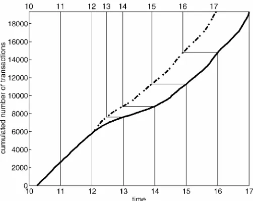
Figure 1. Cumulative Number of Trades, by Daytime (—) and Trans-formed Time (- - -) for the Complete Sample.

are matched against several orders on the other side. On July 4, the market opened late, but we did not exclude this date from our dataset. The average number of trades per day is 458, with a standard deviation of 184. The minimum number of trades on a date is 238; the maximum, 1,022. Ghysels et al. (in press) provided some more information on the Paris Bourse structure. The mean duration in our sample is 53.2 seconds, with a standard deviation of 84.8 seconds. For each time between 10:15A.M. and 17:00P.M., the continuousline in Figure 1 plots

the cumulative number of trades over all days. Hence the slope of the line reects the average trading intensity (over all days) at a certain moment during the day. From Figure 1, it is clear that the average trading intensity is almost constant during the day, with lunchtime as an important exception. During lunchtime, there is a clear attening of the average trading intensity. The lower market activity is pronouncedly present in our dataset; therefore, we must consider a mean duration function that is slightly more complicated than (4). We use the following spec-ication:

ÃiD®C±diC¯xiC° Ãi¡1; (20) where di is an indicator for lunchtime. This extension seems to be sufcient, for the case at hand, because the trading in-tensity is almost constant before noon and after 2:30 P.M.

We set diD1 for transactions that occur between noon and 1:15P.M. Note that the exponentialsmoothing parameter° will take care of a smooth transition of the “normal” intensity to the lower lunchtime intensity. By the same effect, the inten-sity will increase again after 1:15P.M. This gradual change is seen in Figure 1 as the S-shaped form of the cumulative in-tensity around lunchtime. Engle (2000), considering IBM data, adopted a nonparametric specication of the constant in the conditional mean duration equation. There the expected dura-tions uctuate in a more pronounced way over the day, and the simple approach (20) would fail. As long as one is interested in the parameters¯ and°, this nonparametric approach could also be adopted in our current setup.

(9)

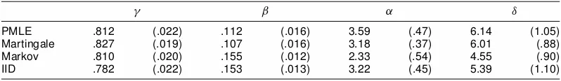
Table 1. Estimates of the Parameters in the ACD Model (20) for the Alcatel Data Based on the Four Procedures Described in the Main Text

° ¯ ® ±

PMLE .812 (.022) .112 (.016) 3.59 (.47) 6.14 (1.05)

Martingale .827 (.019) .107 (.016) 3.18 (.37) 6.01 (.88)

Markov .810 (.020) .155 (.012) 2.33 (.54) 4.55 (.90)

IID .782 (.022) .153 (.013) 3.22 (.45) 5.39 (1.10)

NOTE: “PMLE” refers to the pseudolikelihood method based on an exponential innovation distribution. “Martingale” is the estimator where conditional

distributions are assumed to be based on past innovations. “Markov” is the efcient semiparametric estimator in case the innovation’s distribution is only affected by the last innovation. “IID” refers to the optimal semiparametric estimator in the model where the innovations are assumed to be independent over transactions. Robust standard errors are reported in parentheses; see the text for details.

As mentioned before, our theoretical results rely on a cor-rectly specied mean durationÃiin (20). To assess the accuracy of our specication informally, the dotted line in Figure 1 shows the cumulative number of trades against the transformed time axis in the top of the gure. The time transformation is based on estimated expected duration calculated according to (20). In particular, given the estimated values of®,¯,°, and±, we cal-culate the expected value ofÃiusing the recursion

EÃ0D ®

1_¡¯_¡° and

EÃiD®C±diC.¯C° /EÃi¡1;

where diD1 if theith trade lies between noon and 1:15P.M. anddiD0 otherwise. Given these estimated expected durations, rescaled durationsx¤_i _DxiE_EÃ_Ã0_i are calculated from the durations

xifor each day. The dotted line in Figure 1 is obtained as the cu-mulative number of trades based on these rescaled durationsx¤_i.

The top time axis gives the corresponding time change, which can be informally written asdt¤_DE_EÃ_Ã0

i dt. The transformed in-tensity estimate is almost constant. This shows that our spec-ication of the expected duration picks up the salient features of the data at hand. It is important to note that, except for the introductionof the lunchtime dummydi, we do not enhance the specication of the conditional mean durationÃior apply any preanalysis transformation to the data.

We estimated the ACD model using the PMLE method and three semiparametric methods. The rst estimator (indicated by “Martingale”), uses the score (16) where the conditional vari-ance of the innovations is estimated by a Nadaraya–Watson nonparametric regression of the squared innovationson the pre-vious innovation"i_¡1only, using the procedure outlined in

Sec-tion 3.2. Such an approach is often followed in practice, even if theoreticallythe conditionalvariance in the optimal generalized method of moments (GMM) score (16) depends on the whole past, that is,"i_¡1; "i_¡2; : : :. The second semiparametric estima-tor is based on a Markov assumption for the innovations"i; see Example 2. Again, unknown conditional densities in the efcient score function, in this case (15), are estimated using kernel techniques, and this estimation does not affect the as-ymptotic semiparametric efciency of the estimator. The esti-mator thus obtained is denoted “Markov.” The third semipara-metric estimator imposes independence of the innovations,that is H_i_{D f}?; Ä_g, without specifying the exact distribution; see the efcient score (14) in Example 1. This estimator is denoted by “IID,” and its theoretical properties in the general non-iid semiparametric model are unknown, but there is no reason to

expect that even an elementary property as consistency is pre-served. Because the analysis of the residuals later in this section clearly shows that the innovations are unlikely to be indepen-dent, the IID estimator is only given for comparison and not discussed further. Results of all four estimators for the Alcatel data are presented in Table 1.

Table 1 shows that the semiparametric procedures Martingale and Markov provide smaller standard errors than the pseudo-likelihood estimator. Generally speaking, the gain is equivalent to an increase in the number of observationsby about 30%. This number is obtained as the average relative efciency of the Mar-tingale estimator and the Markov estimator with respect to the PMLE. The GMM-type Martingale estimator and the efcient semiparametric estimator in the Markov model Markov behave similarly for the data at hand. A concern is a possible bias in the Markov estimates for the long-term levels of the durations as measured by®and±in (20).

It is known that estimates for the Fisher information in semi-parametric models often have weak convergence properties. Therefore, we do not base the standard errors in Table 1 on the estimated Fisher information directly; rather, we apply a re-sampling technique. For each day, estimates of the parameters are separately obtained. The estimates and standard errors are based on the location and dispersion of the daily estimates. As-suming that the model innovations are independent over differ-ent days, this gives consistdiffer-ent estimates for the standard errors. Whether the true independence in the data is sufcient to apply this technique is an empirical issue that lies outside the scope of the present investigation.We use the median and the median absolute deviation as measure for location and dispersion, to prevent a dominatingeffect of outlyingdaily estimates. The me-dian absolute deviationis standardized such that in cases of nor-mality, the standard deviationis obtained. Note that, on average, the daily estimates are based on approximately 500 observa-tions. Of course, an alternative would be to use a bootstrap-type procedure, but the theoretical properties of such an approach would be difcult to establish in our non-iid situation, and the computational effort involved would be enormous.

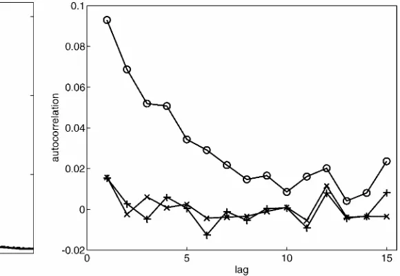
To assess the source of the gain of the semiparametric proce-dures over the pseudolikelihood procedure, we study the resid-uals from the pseudolikelihoodprocedure. Figure 2 plots an es-timate of the unconditionaldensity of the innovations,together with a standard exponential density. Engle (2000) found a sim-ilar graph (see his g. 1) and the data suggest a nonexponential marginal distribution. To study the dependencies between the innovations, Figure 3 shows the autocorrelation function of the residuals, the squared centered residuals, and the log-residuals.

(10)

Figure 2. Comparison of the Estimated Unconditional Density (—) and the Standard Exponential Density (- - -) of Innovations.

We clearly see that both residuals and their squares are (almost) uncorrelated, whereas the log-residuals show a small, but sig-nicantly positive autocorrelation. The proposed semiparamet-ric procedure effectively takes such dependencies into account. The rst-order autocorrelation of log-residuals is only about .094. Apparently, such low dependencies still show up in the efciency gains for the semiparametric estimators. Of course, another possibility could be that the conditional mean is mis-specied. In that case, a nonparametric specication of the con-ditional mean could resolve the problem.

5. SIMULATION RESULTS

The results in the previous section indicate that even small dependencies in the innovations as measured by, for exam-ple, the autocorrelation of the log-residuals can induce sizeable efciency gains of efcient semiparametric procedures over pseudolikelihoodprocedures. In this section we investigate this phenomenon in more detail. We consider parametric models that mimic the most salient features of the Alcatel data. We do not advocate to use these parametric models as an alternative to the semiparametric models introduced in Section 2.2, because misspecication is quite likely and may adversely affect the es-timators. The parametric models in this section are used merely to conrm the properties of the semiparametric estimators in realistic settings.

The residuals of the Alcatel durations in Section 4 show some delicate dependencies. Clearly, the model specication requires that the residuals be uncorrelated. Squared residuals also appear uncorrelated, whereas logarithmic residuals show some weak, but signicant rst-order autocorrelation. An ex-tension of the classical gamma (including the exponential) or log-normal specications incorporating these stylized features is obtained by making the parameters of those distributions time-varying. As an example, consider the possible specica-tion

"i»0.¾_i¡_¡21; ¾i¡¡21/ (21)

Figure 3. ACF of Residuals (_C), Squared Centered Residuals (_£), and Log-Residuals (

±

).

or

"i_»LN

³

¡1₂log.1_C¾_i2_¡₁/;log.1_C¾_i2_¡₁/

´

; (22)

with

¾_i2_¡₁_D:10_C:90"i_¡1:

Note that for both specications, the conditional variance of the innovations is indeed given by¾_i2_¡₁. Clearly, the forego-ing specications are not the only parametric ones that generate dependence structures comparable to those found in the Alca-tel data. Therefore, we advocate using a semiparametric tech-nique for econometric analysis of the structural parameters in the specication of the conditional expected durationÃi. This seems all the more reasonable because a parametrically mis-specied model of the innovation’s distribution does not pro-duce consistent pseudolikelihood estimates in general. As has been pointed out before, this holds also if the parametric spec-ication includes the iid exponential specspec-ication for which pseudolikelihoodprocedures are consistent.

We present results for the same four estimators as used in the analysis of the Alcatel data. The rst estimator (“PMLE”) is the exponential PMLE. For the second estimator (“Martin-gale”), the conditional variance of the innovations may depend in an arbitrary way on the past. The third estimator (“Markov”) is based on the efcient semiparametric score (15) and assumes that the innovations follow a Markov process with unknown transition density. The nal estimator (“IID”) is the efcient semiparametric estimator in case the innovations are iid (see Example 1). The true values in (4) are®_D4:50,¯_D:10, and ° _D:80, and we consider both the gamma specication (21) and the lognormal specication (22). The daily number of ob-servations is, in accordance with the average in the Alcatel data, xed at 500. The computational effort in the simulations is substantial. Therefore, the number of replications is limited to 2,500. Again, we present location and dispersion estimates that are based on robust estimates, that is, the median and the me-dian absolute deviation. The reported standard errors are multi-plied byp2;500=43 to make them comparable with the empir-ical results of Section 4.

(11)

Table 2. Simulation Results for the ACD Model (4) With Innovation Structure (21), Where¾2

i¡1D:1C:9"i¡1

Exact scores Estimated scores

° ¯ ® ° ¯ ®

PMLE .804 (.0140) .088 (.0073) 4.48 (.367) .804 (.0140) .088 (.0073) 4.48 (.367)

Martingale .800 (.0113) .093 (.0052) 4.60 (.328) .807 (.0110) .090 (.0052) 4.37 (.315)

Markov .800 (.0113) .093 (.0052) 4.60 (.328) .813 (.0131) .086 (.0059) 4.18 (.372)

IID .803 (.0143) .090 (.0068) 4.57 (.399)

NOTE: See Table 1 for an explanation of the terminology used.

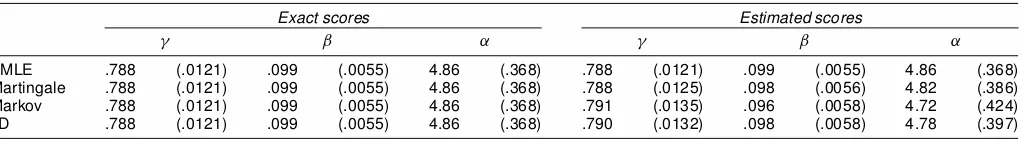
The simulation results for the gamma and the lognormal specication are presented in Tables 2 and 3. For reference, the results in case the innovations are independentlyand identi-cally exponentially distributed are given in Table 4. We present both the estimation results based on exact scores (i.e., as ap-propriate for the data-generating process at hand) and the esti-mation results based on estimated scores. The exact scores are calculated from the relevant formulas in Section 2.3 using the specied densities. From these exact scores, we can then infer the theoretical semiparametric efciency gain and the theoreti-cal ranking of the various semiparametric estimators. The effect of the nonparametric density and regression function estimates follows from comparing the results with exact and estimated scores. Table 4 presents the results in the ideal situation of iid exponential innovations"i. As discussed in Section 3, all four estimators are efcient (even adaptive) in this case. Indeed, the scores used by all estimators are the same, and, consequently, when using exact scores, the estimators are identically equal to the PMLE. In cases where the score functions are estimated, the estimators theoretically still behave the same. The simu-lation results conrm this, because as there is little variation with respect to standard errors. A slight increase in the vari-ation for the semiparametric Markov estimator may be noted, which is caused by the nonparametric conditional density esti-mation therein. The somewhat better behavior of the Martingale estimator over the IID estimator using estimated scores is due to sampling error.

To examine the effect of dependencies on the performance of the estimators, we rst consider the conditional gamma in-novations in (21). In this case, the PMLE and the Martingale and Markov semiparametric estimators provide consistent esti-mates. There is no guarantee (known to us) that the IID semi-parametric estimator is consistent in this setting with dependent innovations.Of course, calculationswith exact scores cannot be performed for this estimator. The results based on exact scores, show that the theoretical standard errors of the PMLE are larger than those of the two consistent semiparametric estimators. This conrms the results of Section 3, because the conditions under which the PMLE provides efcient estimates are not met

in the present simulation where var_f"i_jH_i_¡₁_g _is

nondegener-ate. Note, however, that since the innovations are conditionally gamma distributed, the Martingale and Markov semiparamet-ric estimators are theoretically equal. This follows immediately from plugging in the theoretical conditional gamma density in the efcient score functions in Examples 2 and 3. However, the density estimation required in the implementation of the Markov semiparametric estimator increases its variability to the level of the PMLE, whereas the Martingale estimator retains its theoretical variability.

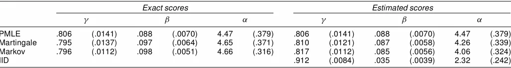
The former two simulations are still quite specic since, as-ymptotically, the Martingale and Markov semiparametric esti-mators coincide. Therefore, we also conducted the analysis us-ing conditionallylognormallydistributed innovationsas in (22). As noted before, the lognormal distribution is not suited as a pseudodistribution in a PMLE procedure, because such an es-timator generally would be inconsistent. However, it is infor-mative to investigate the effect of lognormal innovations on the simulation results; see Table 3. Indeed, as can be seen from the bottom line in Table 3, the last semiparametric estimator (based on an iid-ness assumption on the innovations)does not produce consistent estimates in this case. As before, the Martingale and Markov semiparametric estimators show efciency gains over the exponentialPMLE; however, these estimators are no longer asymptotically equivalent. The table shows an improvement of the Markov estimator, but there also seems to be a bias–variance trade-off. The gains of the efcient semiparametric procedures over the standard exponentialPMLE are, as for the Alcatel data, roughly on an order of magnitude of 30% of the number of ob-servations.

Note that the standard errors for all simulations differ some-what from those found for the Alcatel data. This suggests that in the Alcatel data, even more complicated dependencies than those studied in this section play a role. Clearly, the use of semi-parametric techniques avoids misspecication problems inher-ently present when using parametric models. Note that the sim-ulation results for the Martingale and Markov semiparametric estimators are quite similar in all cases. Apparently, for the

Table 3. Simulation Results for the ACD Model (4) With Innovation Structure (22), Where¾_i2_¡₁D:1C:9"_i_¡₁

° ¯ ® ° ¯ ®

PMLE .806 (.0141) .088 (.0070) 4.47 (.379) .806 (.0141) .088 (.0070) 4.47 (.379)

Martingale .795 (.0137) .097 (.0064) 4.65 (.371) .810 (.0121) .087 (.0058) 4.26 (.339)

Markov .796 (.0112) .098 (.0051) 4.66 (.316) .817 (.0112) .085 (.0056) 4.06 (.324)

IID .912 (.0084) .035 (.0039) 2.32 (.242)

(12)

Table 4. Simulation Results for the ACD Model (4) With IID Exponential Innovations

° ¯ ® ° ¯ ®

PMLE .788 (.0121) .099 (.0055) 4.86 (.368) .788 (.0121) .099 (.0055) 4.86 (.368)

Martingale .788 (.0121) .099 (.0055) 4.86 (.368) .788 (.0125) .098 (.0056) 4.82 (.386)

Markov .788 (.0121) .099 (.0055) 4.86 (.368) .791 (.0135) .096 (.0058) 4.72 (.424)

IID .788 (.0121) .099 (.0055) 4.86 (.368) .790 (.0132) .098 (.0058) 4.78 (.397)

specications chosen in this section, the respective scores (15) and (16) are close.

Summarizing, the simulations conrm that signicant ef-ciency gains may be obtained from the use of semiparametric procedures. We prefer the theoretically optimal semiparametric estimators. Even if large numbers of observations are available for the study of intraday durations, the semiparametric proce-dures allow for much more precise empirical analysis and pre-diction. Moreover, with large datasets the distortions induced by the nonparametric density estimation are likely to disappear. Recall that our results are based on a moderate sample of only 500 observations.

6. CONCLUDING REMARKS

We have discussed optimal estimation in semiparametric du-ration models. The models differ in the specication of the possible dependencies between the innovations. These speci-cations range from the case where innovations are iid with unknown density to completely arbitrary dependencies that only impose an identifying martingale restriction. For these specications, we derived the efcient score functions for the parameters of interest that govern the conditional expected du-ration. We also showed that the often-used exponential PMLE is only efcient under very restrictive conditions and that the other PMLEs (e.g., based on the lognormal or Weibull distribution) are not consistent. We showed that an easily implementable semiparametric estimator allows for signicant (comparable to 30% of the observations) efciency gains. To nd a possible explanation for this phenomenon, we set up a simulation experiment with time-varying parameters in the innovation’s distribution. The stylized features of the Alcatel data for our observation period are mimicked in this experi-ment. These simulations conrm the fact that the semiparamet-ric procedures outperform pseudolikelihoodprocedures.

ACKNOWLEDGMENTS

We thank Joann Jasiak for kindly providing the data. Sev-eral helpful remarks have been given by Rob Engle and Neil Shephard at the.EC/2meeting in Madrid (1999). Finally, two

referees providedvaluable comments. The rst author acknowl-edges support from the European Commission through the Hu-man Potential Programme, Statistical Methods for Dynamical Stochastic Models (DYNSTOCH).

[Received May 2001. Revised April 2002.]

REFERENCES

BIC KEL, P. J. (1982), “On Adaptive Estimation,”The Annals of Statistics, 10,

647–671.

BIC KEL, P. J., KLAAS SEN, C. A. J., RITOV, Y., and WELLNER, J. A. (1993),

Efcient and Adaptive Statistical Inference for Semiparametric Models, Bal-timore: Johns Hopkins University Press.

DROST, F. C., and KLAAS SEN, C. A. J. (1997), “Efcient Estimation in Semi-parametric GARCH Models,”Journal of Econometrics, 81, 193–221.

DROST, F. C., KLAAS SEN, C. A. J., and WERKER, B. J. M. (1997), “Adaptive Estimation in Time-Series Models,”The Annals of Statistics, 25, 786–818. ENGLE, R. F. (2000), “The Econometrics of Ultra-High-Frequency Data,”

Econometrica, 68, 1–22.

ENGLE, R. F., and RUSSELL, J. R. (1998), “Autoregressive Conditional

Dura-tion: A New Model for Irregularly Spaced Transaction Data,”Econometrica, 66, 1127–1162.

GHYS ELS, E., GOUR IEROUX, C., and JASIAK, J. (in press), “Stochastic Volatility Duration Models,”Journal of Econometrics.

GONZÁLEZ-RIVERA, G. (1997), “A Note on Adaptation in GARCH Models,”

Econometric Reviews, 16, 55–68.

GOUR IEROUX, C., and JASIAK, J. (2000), “Nonlinear Autocorrelograms; An Application to Intertrade Durations,” unpublished manuscript.

HÁJE K, J. (1970), “A Characterization of Limiting Distributions of Regular Estimates,” Zeitschrift für Wahrscheinlichkeitstheorie und Verwandte Ge-biete, 14, 323–330.

KOUL, H. L., and SCHICK, A. (1997), “Efcient Estimation in Nonlinear Au-toregressive Time Series Models,”Bernoulli, 3, 247–277.

KREIS S, J.-P. (1987a), “On Adaptive Estimation in Stationary ARMA Processes,”The Annals of Statistics, 15, 112–133.

(1987b), “On Adaptive Estimation in Autoregressive Models When There Are Nuisance Functions,”Statistics & Decisions, 5, 59–76.

LECAM, L. (1986),Asymptotic Methods in Statistical Decision Theory, Berlin: Springer-Verlag.

LINTON, O. (1993), “Adaptive Estimation in ARCH Models,”Econometric Theory, 9, 539–569.

NEWEY, W. K. (1990), “Semiparametric Efciency Bounds,”Journal of Ap-plied Econometrics, 5, 99–135.

STEIGERWA LD, D. G. (1992), “Adaptive Estimation in Time Series Regression Models,”Journal of Econometrics, 54, 251–275.

STEIN, C. (1956), “Efcient Nonparametric Testing and Estimation,” Proceed-ings of the Third Berkeley Symposium on Mathematical Statistics and Prob-ability, 1, 187–195.

VAN DE RVAART, A. (1998),Asymptotic Statistics, Cambridge, U.K.: Cam-bridge University Press.

WEFELMEYER, W. (1996), “Quasi-Likelihood Models and Optimal Infer-ence,”The Annals of Statistics, 24, 405–422.

ZHANG, M. Y., RUSSELL, J. R., and TSAY, R. S. (2001), “A Nonlinear Autoregressive Conditional Duration Model With Applications to Financial Transactions Data,”Journal of Econometrics, 104, 179–207.