Full Terms & Conditions of access and use can be found at
http://www.tandfonline.com/action/journalInformation?journalCode=ubes20
Download by: [Universitas Maritim Raja Ali Haji] Date: 11 January 2016, At: 22:46
Journal of Business & Economic Statistics
ISSN: 0735-0015 (Print) 1537-2707 (Online) Journal homepage: http://www.tandfonline.com/loi/ubes20
Job Durations With Worker- and Firm-Specific
Effects: MCMC Estimation With Longitudinal
Employer–Employee Data
Guillaume Horny , Rute Mendes & Gerard J. van den Berg
To cite this article: Guillaume Horny , Rute Mendes & Gerard J. van den Berg (2012) Job Durations With Worker- and Firm-Specific Effects: MCMC Estimation With Longitudinal Employer–Employee Data, Journal of Business & Economic Statistics, 30:3, 468-480, DOI: 10.1080/07350015.2012.698142
To link to this article: http://dx.doi.org/10.1080/07350015.2012.698142
Published online: 20 Jul 2012.
Submit your article to this journal
Article views: 306
Job Durations With Worker- and Firm-Specific
Effects: MCMC Estimation With Longitudinal
Employer–Employee Data
Guillaume H
ORNYBank of France, DGEI-DEMS-SAMIC, 75 049 Paris Cedex 01, France, and Department of Economics, Universit ´e Catholique de Louvain ([email protected])
Rute M
ENDESInternational Training Centre of the ILO, Turin, Italy ([email protected])
Gerard J.
VAN DENB
ERGDepartment of Economics, University of Mannheim; Institute for Evaluation of Labour Market and Education Policy, Uppsala, Sweden; Department of Economics, VU University Amsterdam, 1081 HV Amsterdam, The Netherlands; Institute for the Study of Labor, Bonn, Germany ([email protected])
We study job durations using a multivariate hazard model allowing for worker-specific and firm-specific unobserved determinants. The latter are captured by unobserved heterogeneity terms or random effects, one at the firm level and another at the worker level. This enables us to decompose the variation in job durations into the relative contribution of the worker and the firm. We also allow the unobserved terms to be correlated in a model that is primarily relevant for markets with small firms. For the empirical analysis, we use a Portuguese longitudinal matched employer–employee dataset. The model is estimated with a Bayesian Markov chain Monte Carlo (MCMC) estimation method. The results imply that unobserved firm characteristics explain almost 40% of the systematic variation in log job durations. In addition, we find a positive correlation between unobserved worker and firm characteristics.
KEY WORDS: Assortative matching; Dynamic models; Frailties; Gibbs sampling; Job transitions; Matched employer–employee data.
1. INTRODUCTION
The basic stylized facts regarding job durations are well es-tablished. For example, the survey by Farber (1999) provides abundant evidence that in OECD (Organisation for Economic Co-operation and Development) countries, long-term employ-ment relationships are common, most new jobs end early, and the probability of a job ending declines with tenure. Unob-served heterogeneity in the probabilities of job exit can largely account for these stylized facts. If workers are heterogeneous in terms of mobility propensities, then the observed job exit rate at any point in time depends on the proportions of those types. Higher-mobility workers experience several short spells, while lower-mobility workers engage in fewer but longer employment relationships. The fact that most new jobs end early is explained by a sufficiently large proportion of high-mobility workers. The fact that the probability of job ending is observed to decline with tenure is then explained by dynamic selection on unobservable characteristics of the workers.
Since job exit is a decision that involves both the worker and the firm, it is plausible that exit rates are affected simul-taneously by characteristics of workers and by characteristics of firms. Whereas the relevance of worker heterogeneity in job durations is well established (see, e.g., Farber1999; Bellmann, Bender, and Hornsteiner2000; and Del Boca and Sauer2009), the empirical evidence on the importance of firm heterogene-ity is much more limited. Abowd, Kramarz, and Roux (2006)
included unobserved worker and firm heterogeneity in a model for wages and job mobility and concluded that there is a large amount of heterogeneity among firms and their tenure profiles. Frederiksen, Honor´e, and Hu (2007) analyzed job durations in a framework with unobserved firm heterogeneity only, and they showed that the latter is an important determinant of the vari-ation in job durvari-ations. Mumford and Smith (2004) estimated linear models for tenure allowing for individual and workplace effects. The results emphasize the importance of allowing for workplace effects.
For a number of reasons, it is relevant to know the relative contributions of worker and firm characteristics as determinants of job durations. First, notice that inequality in society depends on the variation in the characteristics of the jobs that employed individuals have. If the variation in job durations is primarily driven by worker characteristics, then the ensuing inequality will be more persistent. Conversely, if the variation is primar-ily driven by firm characteristics, then the restructuring of the market form in a sector can have large effects on inequality in society. Second, the results of the analysis are of importance for the econometric analysis of job durations. If unobserved firm heterogeneity is important, then the inclusion of very large
© 2012American Statistical Association Journal of Business & Economic Statistics
July 2012, Vol. 30, No. 3 DOI:10.1080/07350015.2012.698142
468
numbers of worker characteristics to a job duration model does not remove the need to deal with unobserved heterogeneity. Third, the results simply help in improving our understanding of the determinants of job durations and job mobility. (In the fol-lowing, we also discuss the relevance of assortative job matching for the study.)
In this article, we estimate multivariate hazard models for job exits (or, equivalently, job durations), allowing for worker-specific and firm-worker-specific unobserved determinants. Worker-specific determinants encompass the propensity of the worker to leave or lose a job, while firm-specific determinants can reflect the firm’s preference to employ a stable workforce. Furthermore, we allow the unobserved effects of matched firms and workers to be correlated. To our knowledge, this is the first study that allows for such a flexible modeling of job mobility. Obviously, the econometric analysis requires observation of multiple job spells per worker and/or multiple job spells per firm. A firm is cross-sectionally and longitudinally connected to multiple workers, whereas a worker is longitudinally connected to mul-tiple firms. We use a matched employer–employee dataset in which both workers and firms are longitudinally followed. The data are from Portugal and are exhaustive for the private sector. The estimates of the correlation between the worker-specific and the firm-specific unobserved heterogeneity term are infor-mative on the extent to which specific types of firms match with specific types of workers. To see this, consider a firm where the job durations are typically short. Is this only because of high job exit rates at the firm, or is it also because the firm attracts workers who have high job exit rates anyway, that is, who would also have high job exit rates if employed at firms where job spells are typically long? The former reflects firm heterogeneity, whereas the latter leads to a positive correlation estimate. Our article is therefore connected to the expanding literature on assortative matching of workers and firms. Recent advances in this literature focus on assortative matching in terms of (worker-specific and firm-specific) productivity (see Lopes de Melo (2008) and Mendes, van den Berg, and Lindeboom (2010), for empirical analyses based on matched employer–employee data). See also Abowd et al. (2004), Andrews et al. (2008), and Woodcock (2008) for fixed-effects panel data analyses of linear wage equations with fixed effects for workers as well as firms.
In the econometric analysis, we treat the unobserved het-erogeneity terms as random effects, one at the firm level and another at the worker level. This is in line with econometric du-ration analysis with unobserved heterogeneity (see van den Berg 2001). Due to right-censoring, fixed-effect panel data methods are not feasible. More to the point, we are interested in the rel-ative contributions of workers’ and firms’ characteristics in the variation of job durations, and the estimation of the distribution of the random effects enables such a decomposition.
The model structure is such that the unobserved worker and firm effects are neither nested nor independent. Our model thus relates to the literature on multiple nonnested random effects. As long as the effects are mutually independent, crossed random-effects models are extensions of nested random-effects models, and they can be fitted using the same procedures. However, with general dependence, the implementation is com-putationally more demanding since the data cannot be grouped in independent blocks (Tibaldi2004). Applications of crossed
random-effects models in a generalized linear model framework include Raudenbush (1993), Van den Noortgate, De Boeck, and Meulders (2003). Because of the complex nonlinear connections between the unobserved individual-specific and firm-specific effects and the observed outcomes, we estimate the models us-ing a Bayesian Markov chain Monte Carlo (MCMC) approach, based on the Gibbs Sampler and in line with Manda and Meyer (2005). Robert and Casella (1999) provided a survey of MCMC. Dependence between the worker and firm random effect in a given job creates an additional complication. If the correlation between worker and firm effects is sufficiently high, then this can entail that the random effects of different workers at a given firm are correlated, and/or that the random effects of different firms employing a given worker over time are correlated. As we will show, this is an implication of the required positive semidefiniteness of the correlation matrix of the random terms of firms and workers. A dependence across workers at a given firm and across firms having employed a given worker implies that many observed job spells of different workers and firms are statistically dependent. Indeed, if many workers and firms are connected, because firms have many employees and workers move between many different firms, then most firms would have jointly dependent random effects, and most workers would also have jointly dependent random effects. Estimation of such a model would involve an insurmountable computational burden. In some particular cases, we consider restrictions on the cor-relation parameters of the worker and firm random effects that ensure that the correlation matrix of the worker and firm ran-dom effects has the following set of properties: it is positive semidefinite while at the same time the worker random effects are iid across workers and the firm random effects are iid across firms. We conclude that this holds true if the correlation between the worker and firm random effects is restricted to an interval strictly smaller than [−1,1] and if firms are small (and if in the observation window, workers are not highly mobile across many firms). Notice that positive assortative matching may rule out any mobility of workers across firms with widely different productivities. In that case, the correlation may be large within small labor market segments, whereas it is absent for connec-tions across segments.
As we discuss in the following, the Portuguese labor market displays low mobility and a high degree of stratification. More-over, it has relatively many small firms. Hence, the empirical analysis is unlikely to be affected in a major way by the above complication. However, this does not imply that our modeling approach is suitable for any type of labor market, particularly if its workers make frequent job transitions and if many of its firms are large. Positive-semidefiniteness of the correlation ma-trix may then be incompatible with iid worker random effects and iid firm random effects.
We should point out that our article has a connection to some recent studies in the literature on job seniority and wages. Specif-ically, the influential article by Dostie (2005) estimates a model in which job durations and wages are simultaneously modeled in a random-effects setting. His approach has been adopted by, for example, Bagger (2007) and Battisti (2009). These studies are primarily concerned with changes within job durations, and less with the relative contribution of firm-specific and worker-specific determinants of job durations. Accordingly, the models
are richer than ours in terms of the role of wages, but they do not allow for a firm-specific effect. The models do allow the job exit hazard to depend on a worker-specific random effect and a match-specific random effect, where the latter is drawn anew for each separate match between a worker and a firm, but these worker- and match-specific effects are assumed to be indepen-dent across workers in a firm and from each other. Note that in this approach, the match-specific effect is effectively nested in the likelihood contribution of the worker, and all this facilitates the empirical analysis.
The article is organized in six sections. The Portuguese matched employer–employee data are described in Section 2. These data have been used before in a number of studies. See, for example, Vieira, Cardoso, and Portela (2005); Cardoso and Portela (2005); and Mendes, van den Berg, and Lindeboom (2010) for descriptions and analyses of the data and for sum-maries of the Portuguese labor market. Section3 presents the duration models that we estimate. Here we also provide some economic intuition for the existence of assortative matching in job durations. In Section4, we discuss the estimation method and the choice of the prior distributions. The results are dis-cussed in Section5. Section6concludes.
2. DATA
The study is based on Quadros de Pessoal, a longitudi-nal matched employer–employee dataset gathered by the Por-tuguese Ministry of Labor and Solidarity. The data are collected through a report that all firms with registered employees are legally obliged to provide every year. All workers employed by a firm in the month of October are in the data. Coverage is low for the agricultural sector and nonexistent for public adminis-tration and domestic services, whereas the manufacturing and private services sectors are almost fully covered.
An identifier is assigned to every firm when it enters the dataset for the first time, while the identifier of the worker is a transformation of his social security number. Based on these identifiers, one can match workers and firms, and follow both over time to identify job spell durations. Unlike some labor force surveys, the Quadros de Pessoaldo not have details on a worker’s labor market events between consecutive years, nor on the exact timing a job exit took place. We can thus identify transitions of workers between firms occurring in time intervals of 1 year, but not the occurrence of other short spells (job, unem-ployment, or nonparticipation spells) within that time interval.
As of 1994, the Ministry has implemented elaborate checks on the accuracy of the firm identification code. Therefore we use the data covering the period 1994–2000. The dataset com-prises nearly 4 million workers and 385,000 firms. We apply a few conditions on workers, firms, and spells: (a) we discard firms that leave, temporarily or permanently, the market; (b) we exclude workers who are observed in a nonpaid job or in self-employment at some point; (c) we exclude spells with entry before 1994, to avoid initial condition problems; and (d) work-ers older than 55 are discarded. This results in what we call the “full data” covering around 338,000 workers and 55,000 firms. To reduce the computational burden of the estimation pro-cedure, we draw a 3% sample of workers that is as close as possible to the full data in terms of worker and firm observables
and job durations. In particular, within each group formed by the combination of all values of the observables, a 3% random sample is drawn, thus maintaining the proportion of each group. Descriptives of the full data and the 3% sample are presented in Appendices A and B. In both, about 91% of the workers experience only one new job spell in the observation window; about 8% experience two spells, and about 1% experience three spells.
In our model of job transitions, we use the following observed characteristics of the worker: age, gender, and education. Age may capture life-cycle effects, as “job shopping” tends to take place mainly at an early age, when the worker is not aware of his own abilities or of the characteristics of the labor market (Johnson1978). Age is grouped into the following categories: 16–25, 26–35, and 36–55 years old. Education is stratified into primary school, lower secondary, upper secondary, and higher education. We also observe whether the job is a part-time job or not, and the corresponding dummy variable is included as firms facing negative demand shocks may tend to first terminate part-time jobs to minimize the loss of specific human capital. Control variables at the firm level include industry, region, and an indicator for multiple plants. Descriptives of firms’ and work-ers’ characteristics are presented in Appendix B. Finally, we use calendar time as an additional explanatory variable.
3. MODEL
3.1 Discrete-Time Job Duration Model
Since we only observe job entry and job exit on an annual ba-sis, we specify the job duration models in discrete time. Specif-ically, we use the time-aggregated mixed proportional hazard (MPH) model for the discrete-time hazard function or condi-tional job exit probability.
At any point in time, an existing firm has one or more work-ers, and these workers change between firms when they move to another job. A firm is thus cross-sectionally and longitudinally connected to multiple workers, whereas a worker is longitudi-nally connected to multiple firms. This means that there is no hierarchical structure between workers and firms.
We denote by i=1, . . . , I the firm index and by j =
1, . . . , J the worker index. We observe all existing worker–firm combinations at one point in time for every calender year in the observation window. As a result, job durations are realized in discrete timek=1, . . . , K.
The hazard function corresponding to individualjin firmi
at elapsed job durationkis the conditional probability of a job termination at this durationk. It depends on (1) the elapsed du-rationk, on (2) worker- and firm-specific observed explanatory variablesxk
ijthat are potentially time varying, on (3) unobserved
characteristics of firmi, and on (4) unobserved characteristics of the workerj. We summarize (3) and (4) by their hazard ef-fects vi andwj, respectively. The firm effect vi is invariant
across job spells at the firm. It may arise for several reasons, in-cluding cross-firm variation in labor contracts, tenure profiles, workforce management policies, and product market conditions or monopsony power. The worker effectwj is invariant across
different jobs occupied by the worker. As noted in the introduc-tion, the existence of such an effect has been demonstrated in
many empirical studies. Both effects are time-invariant. In line with survival analysis or biostatistics, they may be referred to as “unobserved heterogeneity” terms or “frailties.”
In the empirical analysis, we estimate a range of model speci-fications. The simplest model accounts for observed heterogene-ity only. The second specification introduces a worker-specific effect in this simplest model. The third specification allows for worker- and firm-specific effects that are independently dis-tributed of each other. Finally, the most general specification allows the two effects to be correlated within a pair of a worker and a firm.
Following Kalbfleisch and Prentice (1980), the discrete-time MPH model without unobserved heterogeneity is defined as
λk|xkij, β0k,β1
=1−exp−expβ0k+xkijβ1
, (1)
With worker-specific unobserved heterogeneity, we obtain
λk|xkij, β0k,β1, wj
A discrete-time model with two frailties is defined as
λ
likelihood contributions of job spell durations are based on the probability (density) of a possibly right-censored duration con-ditional on the observed and unobserved explanatory variables. With censoring atk, this equals
k
s=1
(1−λij s), (4)
whereas in case of a spell completion at durationk,
λij k k−1
s=1
(1−λij s). (5)
The “full likelihood” is the product of the above expressions for all observed job spells of the workers and firms in the sample. Notice that this full likelihood is defined as a function of the parameter vectorsβ0,β1and the unobserved worker and firm
effects.
The vector of unobserved worker and firm effects has a distri-bution in the population. As we sample workers upon inflow into jobs, and we follow workers over time after that, we effectively take this inflow of workers to be the underlying population. Hence, the sample constitutes a random sample of workers from this population, and it is appropriate to argue that the worker effects wj are marginally iid. If we regard firms as infinitely
exchangeable, then by De Finetti’s theorem, the firm effectsvi
can be modeled as iid conditional on a latent variable. This does not automatically imply that they are marginally iid. To proceed, we make the further assumption that the firm effects are iid as well. In addition, for the remainder of this section, we assume that the firm effectsviare independent of the worker effectswj.
In Section3.3, we incorporate dependence betweenwj andvi.
Notice that the “random effects assumption” states that the frailties are independent of the observed explanatory variables
in the population. This is clearly restrictive. Decisions of indi-viduals and firms may be reflected by the values of the frailties, and these decisions may depend on the relevant values of x. However, contrary to linear models and some nonlinear models for panel data, the identification of duration models with unob-served heterogeneity typically warrants an assumption thatxis independent of unobserved heterogeneity. A detailed survey of the identification of such models was provided by van den Berg (2001). In case the data contain multiple spells sharing the same unobserved determinants, the independence assumption can be discarded. However, in our case, this would amount to observing multiple spells of the same worker in the same firm, which is very unlikely to occur. It is conceivable that such multiple-spell data requirements are unnecessarily strong to be able to relax the assumption thatxis independent of the frailties. We address this issue in a rather modest way, by reestimating the model with samples in which multiple spells per worker and/or per firm are over-represented. Given our limited observation window, this entails an over-representation of short spells. Admittedly, it is also conceivable that allowing for dependence between the worker frailty and the firm frailty will make it more difficult to relax the assumption that both frailties are independent of x. Clearly, the identifiability of duration models with nonnested dependent frailties is an important topic for further research.
Notice that we implicitly assumed that for a given worker, the firm effects in consecutive jobs are drawn from an identi-cal distribution. Economic models of search on the job predict that workers move to better jobs as they become older. In that case, the job exit rate decreases with each successive job. This suggests that the firm effects are systematically decreasing with each successive job. We do not allow for this because it compli-cates the analysis dramatically. First, the ensuing joint distribu-tion of job duradistribu-tions would need to satisfy specific features (see, e.g., van den Berg and Van Vuuren2003). Second, inference on the correlation between worker and firm effects would be more difficult (see Section3.3). Third, we would face an unsolvable initial conditions problem, as our data do not provide job spells dating back to the labor market entry of the workers. The as-sumptions that we make instead are in line with the literature in which matched employer–employee data are analyzed to study wage determinants. Typically, it is assumed that a job-to-job de-cision consists of two dede-cisions that are made sequentially: a job separation and a job acceptance, where the characteristics of the new job are unrelated to those of the previous job, conditional on the observed and fixed unobserved characteristics of the worker. This keeps the empirical inference manageable, and, at least, it constitutes a transparent condition for model identification.
3.2 Behavioral Explanations for Correlated Worker and Firm Effects
In the most extensive version of the empirical model, we allow the worker-specific effect wj on the job duration and
the firm-specific effectvi on the job duration to be correlated.
A nonzero correlation betweenwj andvi in jobs reveals that
assortative matching takes place between workers and firms. Broadly speaking, there are two sets of possible explanations for this. First, the assortative matching is driven by an inherent preference for high or low job durations in both workers and
firms. Second, job stability is correlated to another variable that triggers assortative matching. In the latter case, this may be a more fundamental job characteristic, or it may be some other omitted variable. We discuss these possible explanations in some more detail.
Consider the first explanation. It is possible that job stability as such is deemed valuable by both workers and firms, or at least by a fraction of them. The job matching process may then lead to an alignment of preferences. For example, some firms may have a stable product market and may value long-run relationships between sales employees and customers. It is also possible that some jobs warrant high job-specific human capital investments. At the same time, some workers may have a stronger preference for stable jobs than others. For example, some workers may be more risk averse than others. In these cases, workers and firms with similar preferences may sort themselves into matches with each other.
An example of the second explanation is inspired by the liter-ature mentioned in Section1on assortative matching between workers and firms. This literature focuses on the matching of high-productivity workers with high-productivity firms. Such matches are usually in their joint interest if the production func-tion is supermodular. In a perfectly competitive labor market, the equilibrium results in perfect sorting in terms of productiv-ity, but this does not provide a reason for why the job durations would be sorted as well. Now suppose that it takes a certain amount of time for workers and firms to learn about each oth-ers’ productivity after the job has started. Then one would expect that the matches where both the workers’ and firms’ productiv-ities are relatively high will lead to stable jobs, whereas other matches are sometimes insufficiently attractive for at least one participant to be sustainable. Suppose, in addition, that idiosyn-cratic job separation rates are decreasing in the productivity of the worker and/or firm. Then what we observe in terms of job durations is that the workers and firms that have low job exit rates often form matches. In sum, the worker and firm effects
wj andviare positively correlated.
Another example of the second explanation relies on a more mechanical omitted-variable argument. Suppose that each value of the vector of observed explanatory variablesxcaptures a sep-arate labor market. It may be that within each of these markets there are submarkets (e.g., local regions) with their own degree of labor market volatility. In that case, workers with low job exit rates are often employed at firms with low job exit rates, simply because the job duration is a proxy for unobserved local market characteristics.
3.3 Modeling of Correlated Worker and Firm Effects
We may capture the dependence betweenvi andwj by the
correlation matrix associated with the vector of all vi andwj
in the population. Recall that the vi are independent across
firms and thewj are independent across workers. In principle
one may consider flexible correlation patterns between worker and firm effects, for example, by allowing some worker effects to be more strongly correlated with a certain firm effect than other worker effects. However, it is clear that parsimony is im-portant to prevent the number of parameters from exploding. Smith and Kohn (2002) and Liu, Daniels, and Marcus (2009)
developed parsimonious Bayesian approaches to estimate the covariance matrix generated by multivariate Gaussian longitu-dinal processes. However, these studies do not examine matri-ces of dimension over (30×30), and it is unclear whether such larger dimensions can be handled by these methods. Raknerud (2009) considered a linear wage equation with worker-specific and firm-specific random effects that may be correlated with each other. He developed an estimation method based on a state space representation, under the assumption that terms of order equal to the square of the correlation coefficient can be ignored. This method seems only applicable in a linear-equation setting. To proceed, we assume equicorrelation, that is, corr(vi, wj)=
corr(vi′, wj′)=ρ,∀(i, j)=(i′, j′). This reduces inference on
the correlation matrix to inference on a single parameter ρ. Note that ann×nmatrixRis a correlation matrix ofnrandom variables if and only if the following three conditions are sat-isfied: the matrix is symmetric, its diagonal elements are equal to one, and the matrix is positive semidefinite. The latter prop-erty imposes restrictions on the range of the possible values of the elements of the matrix. In the case of the equicorrelation assumption, this amounts to a restriction on the range of values of ρ. In particular, the condition of positive-semidefiniteness rules out that one random variable is strongly correlated to other random variables that are themselves uncorrelated to each other. As an example, consider one firm withnworkers (or, equiv-alently, one worker withnjobs). Forn=2, the candidate cor-relation matrix of the effects (v1, w1, w2) is defined as this is not compatible withw1 andw2being independent. It is not difficult to show that for a general number of employeesn
of the firm, positive-semidefiniteness is equivalent to
|ρ| ≤ √1
n. (7)
These bounds do not depend on the functional form of the joint distribution. Clearly, the assumption of mutually indepen-dent worker effects and mutually indepenindepen-dent firm effects is not compatible with a strong correlation between worker and firm effects. However, this does not mean that any model with
ρ=0 is misspecified. Consider a labor market where firms are small and where workers are not mobile across different firms in the course of their lifetime. In that case, the above restriction may be satisfied. Similarly, if the labor market is segmented, for example, due to positive assortative matching across segments, and if the segments are small, then the restriction is weaker than may be suggested by (7). With two equally large segments, the correlation matrix (v1, w1, w2, v2, w3, w4) can be expressed as number of workers and firms is now twice as large. In general,
withmequally large segments, inequality (7) is replaced by
|ρ| ≤ √1
n/m. (9)
To avoid confusion, notice that the parameterρdoes not give the overall correlation between worker and firm effects but the within-segment correlation. For segments with small firms and low-mobility workers, the boundary values ofρ are relatively far away from zero.
With complex longitudinal patterns of worker-firm combina-tions, it is difficult to derive precise bounds for admissible values ofρ, and therefore more difficult to assess how likely it is that the model is misspecified. Notice that correlations of observed outcomes across workers and firms may also be explained by common observed determinants that are included as explanatory variables in the model. In the end, it is an empirical question whether, within a market, firms are sufficiently small and worker mobility is sufficiently low, for the assumption of mutually inde-pendent worker effects and mutually indeinde-pendent firm effects to be compatible with certain nonzero values ofρ. Cabral (2007), in his study on the importance of small firms in Portugal, stated that 86% of firms have fewer than 20 employees. In our own data, this number is around 90%, and around 60% of the firms have four employees or less. Of course, firms themselves may be segmented in different parts that have no (or almost no) common determinants of job spell durations, on top of those captured by the observed covariates. Mendes, van den Berg, and Lindeboom (2010) included a brief overview of the Portuguese labor mar-ket. They concluded that in the years covered by our data, it has been much more stable than in other countries. Institutional features and barriers make mobility costly and tend to hamper worker mobility across jobs. In this sense, the Portuguese labor market may be better suited for our modeling approach than the labor markets in other countries.
We therefore include estimation results for the model withρ
as an additional parameter. This approach can be further justi-fied by the low numbers of job spells per worker in the data as described in Section2. Recall that the observation window per worker consists of at most 7 years, and for 99.9% of all workers, we observe less than four job spells. Obviously, with a limited number of spells per worker and per firm, models with nonzero
ρ may not violate the positive-semidefiniteness of the corre-lation matrix for the firms and workers in the data, under the maintained assumption of mutually independent worker effects and mutually independent firm effects.
There is an apparent contradiction between, on the one hand, the requirement that firms are sufficiently small and worker mo-bility is sufficiently low for the model with correlated worker and firm effects to be coherent, and, on the other hand, the use-fulness of a large firm size and worker mobility across firms for the model to be identifiable. Concerning the latter aspect, no-tice that duration models with one-dimensional random effects are identified in the absence of multiple spells per unit. This compares favorably to regression models with one-dimensional random effects and a single observation per unit. However, with single-spell data, inference results are not robust to parametric functional form assumptions in the model (see van den Berg 2001, for an overview). This can be remedied if the observed explanatory variables are time-varying. Our data contain annual
observations of the explanatory variables, so they may vary over time, and our models incorporate this. Recall also that although the fraction of workers with multiple observed spells is small, the size of the dataset is considerable.
If the resulting estimate ofρis large in absolute value, then this may indicate misspecification in the sense that the assump-tion of mutually independent worker effects and mutually inde-pendent firm effects is violated. This assumption is shared by many empirical studies in which job duration models are esti-mated. In this sense, evidence for a large value ofρmay be of importance for empirical studies of job durations with worker data and the empirical analysis of job turnover with firm data, as these types of analyses assume independent outcomes across workers and firms, respectively. Obviously, since we also esti-mate models that imposeρ =0, we can examine whether the fit of the latter model is significantly worse.
Notice that in principle, the above concerns can be avoided by estimating a model in which the assumptions of mutually independent worker effects and mutually independent firm ef-fects are relaxed. This means relaxing the almost universally made econometric assumption that random effects are indepen-dently distributed across subjects. As noted in the beginning of this section, in the most extreme case, if we do not make any assumption on the correlation matrix of the joint distribution of the random effects, the sample data simply provide a single joint observation of a large number of correlated spells, and the number of parameters in the correlation matrix exceeds the sam-ple size. The more modest the relaxation of the assumption of mutually independent worker effects and mutually independent firm effects, the more parsimonious the model. As we have seen, the development and statistical inference of models that are less parsimonious than ours is still in its infancy. The computational burden is substantial. Even with simulation methods one has to draw from a joint normal distribution with a dimension equal to the sum of the number of workers and the number of firms, with a structured variance matrix of which each element has to satisfy a number of constraints increasing with the matrix dimension to ensure its positiveness. In a sensitivity analysis in Section5.4, we report some results based on a model that allows worker effects to have a fixed correlation across workers and firm effects to have a fixed correlation across firms. This increases the range of admissible values of ρ. For example, with one firm and three workers, the positive-semidefiniteness of the correlation matrix implies thatρ≤√(1+2α)/3, with
α >−1/2 being the correlation between worker fixed effects. This is larger than the upper bound in Equation (7) forn=3 for anyα >0. In another sensitivity analysis, we estimate the model with samples that restrict the number of workers per firm. A potentially promising alternative approach could be to define clusters of workers and firms and to use fixed-effects estima-tion methods, see, for example, Sargent (1998) for a univariate analysis.
With the above models, there are a number of reasons to perform inference with Bayesian MCMC estimation methods. First, these methods do not require large-sample asymptotics. Second, these methods do not require numerical integration over multidimensional random effects. Nevertheless, we know that Bayesian approaches for nested random-effects Cox pro-portional hazard models are computationally intensive. With
massive data, the extension to nonnested effects is not trivial (Tibaldi2004); Horny et al.2008). In the next section, we dis-cuss our inferential approach in detail.
4. BAYESIAN INFERENCE
Concerning the functional form for the unobserved hetero-geneity distribution, it is useful to have a family of distributions where the correlation or covariance of the dependence between the worker and firm random effects is a separate parameter that can attain positive as well as negative values. We adopt a normal distribution for the random effects. We normalize the mean to zero, and we denote the variances byσv2forviand byσw2forwj.
Recall that we estimate four model specifications. The sim-plest model accounts for observed heterogeneity only, soσv=
σw=0. The second specification only imposes σv=0. The
third specification allows for nonzeroσv andσw=0 but
im-poses ρ=0. Finally, the most general specification does not impose constraints on the parameters of the bivariate normal distribution. The effect of the misspecification of the functional form of the unobserved heterogeneity distribution has been in-vestigated in detail for discrete duration models. Nicoletti and Rondinelli (2010) showed that an incorrect normality assump-tion for the unobserved heterogeneity distribuassump-tion does not bias the baseline hazard and the covariate parameter estimates.
The Bayesian approach augments the assumed model with the prior beliefs on the parameters. We choose proper but uninfor-mative priors, allowing unlikely values of the parameters to not necessarily have a zero posterior probability. Assigning a zero prior probability to some parameter values would lead to a zero posterior probability, even if the likelihood reaches its maximum at these values. Manda and Meyer (2005) specified a baseline hazard with steps related through a first-order autocorrelated process, and Grilli (2005) used a polynomial specification. Be-cause the time period under study consists of six time intervals, we specify a piecewise constant baseline hazard with unrelated coefficientsβ0k. (We also estimated models using a polynomial specification in preliminary analysis and were led to a 6 degrees polynomial.) The coefficientsβ1associated with thexvariables
are given independent Gaussian priors with means 0 and very large variances 1000.
To complete the specification of the posterior distribution, we must specify a prior distribution for the parameters of the unob-served heterogeneity distribution. The precision of each random effect (i.e.,σ−2
v andσw−2) follows a gamma distribution, that is,
the conjugate prior of the Gaussian distribution, and we base our prior elicitation on descriptive statistics. The annual transition probability per worker is about 3.5% for the 5th percentile of the duration distribution and 0.9% for the 95th percentile. So for 90% of the population, there is at most a four-fold variation be-tween the odds of two workers. The corresponding confidence interval on the transition probability is thus of width 3, which suggestsσw=0.5. We set our prior for the precision σw−2 to
a gamma distribution with expectation 2 and variance 4. Simi-larly, the transition probability per firm is in a range from 1.3%
to 4% for 90% of the population, suggesting a gamma prior with expectation 3 and variance 9 forσ−2
v . Finally, forρ, a
noninfor-mative prior, that is, a uniform distribution, is specified over its range.
Our model is a Bayesian hierarchical model. We first specified the duration model, then the prior distribution, and finally the distributions on the parameters of the priors. Our posterior is not a common distribution, even with all priors being independent. However, we can construct a Markov chain with elements fol-lowing the posterior distribution, and approximate the Bayesian estimator using a Monte Carlo method. Notice that such infer-ence is straightforward if thevi andwj were observed. We use
Gibbs sampling (Gelfand and Smith1990), a data augmenta-tion algorithm, to simulate unobserved heterogeneity terms for all firms and workers. These are used to sample the parameters from the posterior density. In the Technical Appendix, we ex-plain the algorithm in detail. Notice that the approach places distributional constraints on theviandwj through their second
moments. Asσvandσwapproach zero,viandwjget more
con-centrated around 0, indicating homogeneous firms and workers. Conversely, large variances indicate heterogeneous firms and workers. The model thus adjusts to the amount of unobserved heterogeneity in the sample.
5. RESULTS
5.1 Unobserved Heterogeneity
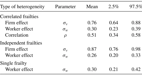
The estimates of the unobserved heterogeneity distributions for the three model specifications as defined in Section4 are reported inTable 1. The estimation results of parameters shared by multiple model specifications are quite similar across the three specifications, meaning that increasing the unobserved heterogeneity complexity does not strongly affect the estimates of those parameters. In the three specifications,σwis estimated
around 0.3 and is significant with posterior standard deviations around 0.04. The estimates ofσvrange from 0.76 to 0.87, with
posterior standard deviations around 0.07. These results provide strong evidence that both variances are effectively nonzero, with the effects of firms’ unobserved characteristics being more dis-persed than those of workers’ unobservables.
The correlation between the worker and firm effects is es-timated to be positive and is highly significant at conventional levels. Notice that the estimated value of 0.51 is reasonably high
Table 1. Estimates of the standard deviations and correlation of the unobserved heterogeneity distributions
Type of heterogeneity Parameter Mean 2.5% 97.5%
Correlated frailties
Firm effect σv 0.76 0.64 0.88
Worker effect σw 0.30 0.23 0.39
Correlation ρ 0.51 0.34 0.58
Independent frailties
Firm effect σv 0.87 0.76 0.98
Worker effect σw 0.26 0.20 0.33
Single frailty
Worker effect σw 0.30 0.21 0.42
Table 2. Estimates of theβcoefficients
Random effects
Variable None Worker Independent Correlated
Elapsed tenure
2 years −0.60 −0.58 −0.27 −0.40
3 years −0.96 −0.93 −0.50 −0.68
4 years −1.36 −1.33 −0.80 −1.00
5 years and more −2.14 −2.09 −1.50 −1.74
Worker’s characteristics
Female −0.25 −0.26 −0.34 −0.31
Age:
16– 25 0.59 0.59 0.76 0.69
26 – 35 0.32 0.32 0.41 0.37
Education:
Primary school 0.33 0.33 0.21 0.17
Lower secondary 0.33 0.33 0.25 0.20
Part-time 0.56 0.57 0.66 0.62
Firm’s characteristics
Multiple plants 0.19 0.20 0.31 0.27
Region:
Center 0.12 0.13 0.19 0.19
Lisbon and Tagus Valley 0.36 0.37 0.45 0.41
Alentejo, Algarve and Islands 0.18 0.19 0.30 0.28
Sector:
Construction 0.38 0.39 0.42 0.37
Trade 0.33 0.34 0.34 0.30
Transports 0.05 0.05 0.32 0.32
Financial 0.67 0.68 0.71 0.60
Constant −2.48 −2.53 −3.08 −2.78
Log-likelihood −7700 −7570 −6135 −6640
Number of workers 9222 9222 9222 9222
Number of firms 6582 6582 6582 6582
NOTES: Coefficients in bold are significant at 5% level. Omitted categories: elapsed tenure is 1 year, male, age 36–55, upper secondary or university education, full-time job, firm only has one plant, northern region, mining, manufacturing, electricity/gas/water sectors. Year dummies are included but not reported since they are all insignificant at the 5% level.
in the light of the discussion in Section3.3. The value does pro-vide strong epro-vidence for positive assortative matching in terms of job exit determinants, but at the same time, it may suggest that the maintained assumption of firm-specific (worker-specific) ef-fects being independent across firms (workers) may be violated. Robustness checks are provided in Section5.4.
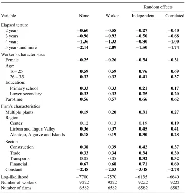
5.2 Observed Heterogeneity
The posterior means for theβcoefficients together with in-formation regarding their significance are reported inTable 2. Negative duration dependence is found to be significant, with the probability of separation declining monotonically with tenure (i.e., with the elapsed duration). This suggests that the empiri-cally observed inverse relationship between separation rates and job tenure would not be fully explicable by pure heterogeneity models that do not account for duration dependence. Notice that the magnitude of the tenure effect reduces once we allow for firm-specific random effects.
Regarding the controlled worker characteristics, we find that women tend to move less. This result contradicts the findings of many previous studies of job mobility. The main reason could be the fact that the gender difference in terms of mobility rates is
changing over time. Light and Ureta (1992) found that women belonging to early U.S. birth cohorts appeared to be more mobile than men but this conclusion is reversed when more recent cohorts are considered.
The results for age are relative to the omitted category of workers aged 36–55 years (the oldest category considered in our study). Thus, they indicate higher transition probabilities for the younger workers. These estimates can be interpreted in the light of on-the-job search models or models of job shopping. The first type of models predicts that, since the match quality is known ex-ante, more experienced workers are less mobile because they had already time/opportunity to move into high-quality matches. Job shopping predicts that mobility decreases with age, as the worker becomes more aware of his own abilities and of the characteristics of the labor market.
Job transitions are also influenced by the education level of the worker. Workers with upper secondary and university ed-ucation (the reference category in our estimates) make fewer transitions. Again, the education effect reduces once we include firm-specific random effects. The estimate of part-time job effect confirms one of the stylized facts of the empirical job duration literature: part-time job status has a strong positive effect on the probability of job separation.
Table 3. Decomposition of total systematic variation of the log durations
Source %
Observed variables 40
Firm unobserved effect 37
Worker unobserved effect 14
Correlation 9
Looking at the characteristics of the firms, we find some dif-ferences across economic sectors and across regions. The North (the reference category) is the region with the lowest job mo-bility, while Lisbon and Tagus Valley is at the other extreme. In fact, Lisbon is the largest city of the country and has the most developed and dynamic labor market. In terms of sectors, the fi-nancial sector exhibits the highest job turnover rates while man-ufacture (the omitted sector) has the lowest ones. The calendar time coefficients (i.e., the year dummies) are always small and insignificantly different from zero (for sake of brevity, they are not reported). This confirms evidence cited in Mendes, van den Berg, and Lindeboom (2010) that our observation window con-stitutes a time of relative stability in the Portuguese labor market.
5.3 Implications
Using the general model specification, we decompose the systematic variation of the log job durations, to quantify the rel-ative importance of its three components: the variation due to the firm unobserved heterogeneity, the variation due to the worker unobserved heterogeneity, and the variation due to the observed explanatory variables. We simulate the variance by drawing the observed and unobserved heterogeneity from the estimated and observed distributions. We obtain a precise approximation of var(logTij k) with a sufficient number of drawings.Table 3
re-ports the results.
The observed characteristics of firms and workers included in the estimated model explain only 40% of the systematic variation of job durations. The remaining variation is mostly explained by the unobserved heterogeneity at firm level. The results indicate that the unobserved components explain more than half of the systematic variation in job durations. Thus, the firm and worker observed explanatory variables are insufficient to capture the heterogeneity in job mobility patterns.
The Bayes factor summarizes the evidence provided by the data in favor of one model over another, and we use it to com-pare the different models. It is the ratio of the probabilities of the data under the different assumed data generating processes (Lan-caster2004). Twice the logarithm of the Bayes factor is on the same scale as the deviance and likelihood ratio test statistics. Fol-lowing the critical values reported in Kass and Raftery (1995), we conclude that there is very strong evidence in favor of models allowing for two-sided unobserved heterogeneity, among which the model with correlated frailties is the strongly preferred one.
5.4 Sensitivity Analysis
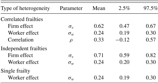
Model specifications allowing for either worker effects or firm effects (or no random effects) can be straightforwardly
Table 4. Estimates of the standard deviations and correlation of the unobserved heterogeneity distributions—multiple spells
over-represented
Type of heterogeneity Parameter Mean 2.5% 97.5%
Correlated frailties
Firm effect σv 0.62 0.47 0.67
Worker effect σw 0.24 0.19 0.30
Correlation ρ 0.33 −0.12 0.57
Independent frailties
Firm effect σv 0.71 0.59 0.82
Worker effect σw 0.24 0.20 0.30
Single frailty
Worker effect σw 0.24 0.19 0.30
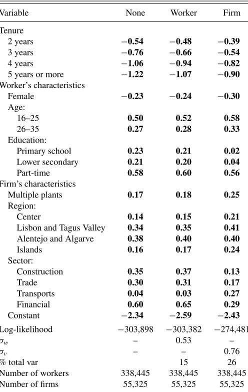
estimated with maximum likelihood estimation using the full population data, without large computational burdens. We use an adaptive Gauss–Hermite quadrature approximations of the mixing distribution when necessary. Results are reported in Appendix C, Table C.1. Theβ estimates are broadly similar to the Bayesian estimates reported in the previous subsections. The likelihood improves with the inclusion of both the worker and the firm effects. Estimates indicate that worker and firm effects variances contribute 15% and 26%, respectively, to total systematic variance, when included separately.
As mentioned in Sections2and3.1, for most workers, we only observe one job spell, and this could potentially make the re-sults sensitive to functional-form assumptions. As an informal robustness check, we reestimate our models in a sample that over-represents workers with multiple spells. From the workers in the full data, we randomly select 2.5% of the workers with single spells and 10% of those with multiple spells. This sam-ple includes 7321 workers and 6906 firms, where 70% of the workers have one spell, 27% of them have two spells, and the remaining 3% have three spells. The estimates of the standard deviations and correlation of the unobserved heterogeneity dis-tributions are reported inTable 4. The standard deviations of worker and firm unobserved effects are close to our main results (inTable 1). In each case,σvis more than twice as large asσw.
The estimate of the correlationρ is somewhat smaller at 0.33, and its precision decreases, so that it is only marginally sig-nificant. Notice that oversampling workers with multiple spells implies that we oversample job matches of lower quality. So, we might expect to find that this affects the estimate of the correlation parameter in this direction.
In additional sensitivity analyses, we use a sample with up to and including three spells per worker and up to and includ-ing three workers per firm, and another sample where these numbers are further reduced to two. If the estimation ofρ is affected by the specification issue discussed in Section3.3, then we expect the estimate ofρ to be smaller when using the re-stricted samples. Due to the small number of spells per worker that are observed in our observation window 1994–2000, the re-strictions do not affect the distribution of the observed worker’s characteristics. It turns out that the estimation results, which are available upon request, are similar to the results in the previous subsections. The estimate of the standard deviation of the firm effect decreases somewhat in the strength of the restriction on
the number of workers per firm. Yet it is always estimated to be larger than the standard deviation of the worker effect. The estimated correlation between the random effects ranges from 0.5 to 0.6 when using the restricted samples, which is very close to the estimate from the unrestricted sample.
We also performed some numerical investigations based on a model with three correlations: one common correlation across the worker random effects, one common correlation across the firm random effects, and our parameter ρ. Interestingly, the resulting estimate of ρ is not larger than in our main results, whereas the estimates of the other correlations are close to zero. This provides some additional evidence for the reliability of our main results.
6. CONCLUSION
This article demonstrates how modern Bayesian MCMC es-timation methods can be fruitfully applied to estimate models of job durations with both worker-specific and firm-specific ef-fects. In such models, the various unobserved worker-specific and firm-specific effects are not nested. We also examine the performance of the approach in case the effects are correlated between worker and firm. This expands the set of methods that can be used for the analysis of mobility and matching.
Our results reject a homogeneous view of the labor market, where firms adopt similar workforce management strategies and individuals have similar job change behavior. Instead, the esti-mates confirm the importance of the unobserved heterogeneity at the individual level, and indicate a large amount of unobserved heterogeneity at the firm level. Indeed, almost 40% of the sys-tematic variation in the logarithm of job durations is due to variation in the effects of unobserved firm characteristics. Mod-eling the unobserved heterogeneity underlying job transitions as coming only from worker observables and unobservables, as is commonly done, is insufficient.
Results for the model allowing for correlation between the two random effects indicate a positive correlation. Thus, empir-ical evidence suggests that employer–employee matching tends to follow an assortative pattern in terms of unobservable charac-teristics of firms and workers—workers and firms with similar outcomes in terms of job mobility and turnover, respectively, tend to match together.
We show that positive semidefiniteness of the correlation ma-trix of the random effects of firms and workers imposes a re-striction on the value of the correlation parameter, under the maintained assumption of marginally iid worker random effects and marginally iid firm random effects. The restriction is strong if, within a market, the firms between which workers move are large. We argue that in our context, this is unlikely to affect the results. However, this does not imply that our modeling approach is suitable for a different type of labor market, partic-ularly if its workers make frequent job transitions and if many of its firms are large. Positive-semidefiniteness of the correlation matrix may then be incompatible with iid worker random effects and iid firm random effects. It is a challenge for future research to extend our contribution, by considering dependence struc-tures between worker and firm random effects that are more widely applicable, and by developing corresponding feasible estimation methods.
As an additional topic for further research, it would be in-teresting to relate our empirical finding of positive assortative matching of job duration determinants to economic models of labor markets with mobility. For example, one may impose or test restrictions from economic models that relate the amount of job search frictions to the wage and the job duration, see, for example, Lise, Meghir, and Robin (2008) for such models.
TECHNICAL APPENDIX: GIBBS SAMPLING ALGORITHM
LetLandLidenote the full likelihood and the contribution to
the full likelihood by all observed job spells of workers at firm
i, respectively, as functions of the parameter vectorsβ0,β1and
the unobserved worker and firm effects. The sampling proceeds as follows:
Generate unobserved heterogeneity terms. ∀i=1, . . . , I, generate the (vi,wi), where wi is the vector of the
un-observed effects of the individuals who ever worked in firmi:
f(vi,wi|β0,β1, σv, σw, ρ)∝φ1+ni(vi,wi)Li, (10)
where φ1+ni is the prior joint density of the unobserved
heterogeneity terms, that is, the multivariate Gaussian den-sity of dimension 1+ni. Recall that both random effects
are assumed to have a zero mean and that the correlation matrix is structured as in Equation (6).
Draw unobserved heterogeneity distribution parameters. Use the simulated unobserved heterogeneity terms to generate
ρfrom
The support ofρis bounded. We use slice sampling (Neal 2003), that generates draws from a distribution by sampling from the region under the plot of the density function. The support ofσ2
v andσw2 is also bounded, and we use slice
sampling to generateσ2
v from
whereaandbare the parameters of the prior distribution
γ(a, b) specified forσ−2
v . Similarly, generateσw2 from its
conditional distribution.
Generate observed heterogeneity parameters. We use the un-observed heterogeneity terms and parameters as inputs when sampling the coefficients of the observed hetero-geneity. Generateβ0k,∀k=1, . . . , K,from
where only the part ofLconcerning the elapsed durationk
is relevant. Finally, in obvious but informal notation, draw
elements ofβ1from
f(β1|β0,v,w, σv, σw, ρ)∝exp
− β
2 1 2σβ1
L. (14)
The density φ1+ni can be simplified as the product of the
marginal distribution of the vi with the distribution of thewj
conditional onv. As the worker effects are supposed to be
mutu-ally independent, this involves univariate Gaussian distributions with E(wj|v)= ρσw
σv
i∈Rjvi, whereRjdenotes the set of firms
where individualjever worked, and var(wj|v)=σ2
w(1−njρ2),
wherenj denotes the total number of firms where individualj
ever worked.
The densities involved do not belong to common distributions, and we use additional samplers inside the Gibbs steps. Steps in-volving draws of the unobserved heterogeneity terms or draws of the observed heterogeneity parameters are performed using an adaptive single component Metropolis algorithm (Haario, Saks-man, and Tamminen1999). Metropolis–Hastings sampler does not mix well when the proposal distribution is not well chosen. This has motivated extensions of the Metropolis–Hastings algo-rithm, such as the slice sampler (Neal2003), to incorporate steps so that the proposal can change during the run. Furthermore, the slice sampler is particularly well suited to sample when the sup-port of the parameters involved is bounded. We thus use it to sim-ulate the parameters of unobserved heterogeneity distribution.
We are interested in statistics, such as means and confidence intervals, computed from draws of the posterior distribution. We thus need the chain of draws constructed by the Gibbs sampler to converge in distribution to the target distribution. We use several criteria to recognize convergence. First, we use trace plots. Second, we run two chains at overdispersed locations for each model, with 50,000 iterations for each model. Convergence implies that within variance of the draws is approximatively equal to the between variance, and we assess it using Gelman and Rubin (1992) statistics. All chains reached an equilibrium within 20,000 iterations. The posterior statistics are computed from the postconvergence iterations.
APPENDIX A: SUMMARY STATISTICS OF THE DURATIONS
Table A.1. Observed uncensored spells
Job spell duration Full data (%) Sample (%)
1 64.0 68.2
2 19.9 19.5
3 9.6 7.9
4 or more 6.4 4.3
Total 100 100
NOTE: Durations are in years.
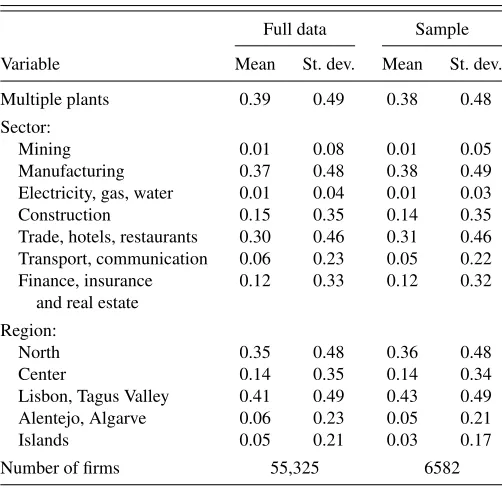
APPENDIX B: DESCRIPTIVES OF THE EXPLANATORY VARIABLES
Table B.1. Firm characteristics
Full data Sample
Variable Mean St. dev. Mean St. dev.
Multiple plants 0.39 0.49 0.38 0.48
Sector:
Mining 0.01 0.08 0.01 0.05
Manufacturing 0.37 0.48 0.38 0.49 Electricity, gas, water 0.01 0.04 0.01 0.03
Construction 0.15 0.35 0.14 0.35
Trade, hotels, restaurants 0.30 0.46 0.31 0.46 Transport, communication 0.06 0.23 0.05 0.22 Finance, insurance 0.12 0.33 0.12 0.32
and real estate
Region:
North 0.35 0.48 0.36 0.48
Center 0.14 0.35 0.14 0.34
Lisbon, Tagus Valley 0.41 0.49 0.43 0.49 Alentejo, Algarve 0.06 0.23 0.05 0.21
Islands 0.05 0.21 0.03 0.17
Number of firms 55,325 6582
Table B.2. Worker’s characteristics
Full data Sample
Variable Mean St. dev. Mean St. dev.
Female 0.38 0.49 0.37 0.48
Age:
16–25 0.34 0.47 0.34 0.47
26–35 0.40 0.49 0.40 0.49
36–55 0.26 0.44 0.26 0.44
Education:
Primary school 0.31 0.46 0.30 0.46 Lower secondary 0.43 0.49 0.44 0.50 Upper secondary 0.27 0.44 0.26 0.44
and university
Part-time 0.08 0.27 0.06 0.24
Number of workers 338,445 9222
APPENDIX C: FREQUENTIST ESTIMATES
Table C.1. Frequentist estimates—full data
Variable None Worker Firm
Primary school 0.23 0.21 0.02
Lower secondary 0.21 0.20 0.04
Part-time 0.58 0.60 0.56
Firm’s characteristics
Multiple plants 0.17 0.18 0.25
Region:
Center 0.14 0.15 0.21
Lisbon and Tagus Valley 0.34 0.35 0.41
Alentejo and Algarve 0.38 0.40 0.40
Islands 0.16 0.17 0.24
Log-likelihood −303,898 −303,382 −274,481
σw – 0.53 –
σv – – 0.76
% total var 15 26
Number of workers 338,445 338,445 338,445 Number of firms 55,325 55,325 55,325
NOTE: Coefficients in bold are significant at 1% level. Omitted categories: elapsed tenure is 1 year, male, age 36–55, upper secondary or university education, full-time job, firm only has one plant, northern region, mining, manufacturing, electricity/gas/water sectors.
ACKNOWLEDGMENTS
We thank the Editor Kei Hirano, an anonymous Associate Editor, two anonymous Referees, Franc¸ois Laisney, Bo Honor´e, Jean-Pierre Florens, Denis Foug`ere, Bertrand Koebel, Franc¸ois Langot, Bart Cockx, and participants in French Economic Asso-ciation (AFSE), Society of Economic Dynamics (SED), Society European Meeting (ESEM), and Institute for the Study of Labor (IZA) conferences, for detailed and helpful comments. We are grateful to the Portuguese Ministry of Employment (Statistics Department) for the access to the data. Mendes acknowledges financial support by the Portuguese Foundation for Science and Technology. The views expressed in this article are those of the authors and do not necessarily reflect the views of the Interna-tional Training Centre of the ILO or the Bank of France. Part of the work was carried out while Horny was at Louis Pasteur Uni-versity in Strasbourg and while Mendes was at VU UniUni-versity Amsterdam and Collegio Carlo Alberto, Turin, Italy.
[Received July 2009. Revised March 2012.]
REFERENCES
Abowd, J., Kramarz, F., Lengermann, P., and P´erez-Duarte, S. (2004), “Are Good Workers Employed by Good Firms? A Test of a Simple Assortative Matching Model for France and the United States,” Working Paper, Cornell University. [469]
Abowd, J., Kramarz, F., and Roux, S. (2006), “Wages, Mobility and Firm Performance: Advantages and Insights From Using Matched Worker-Firm Data,”The Economic Journal, 116 (512), F245–F285. [468]
Andrews, M., Gill, L., Schank, T., and Upward, R. (2008), “High Wage Work-ers and Low Wage Firms: Negative Assortative Matching or Limited Mo-bility Bias?,”Journal of the Royal Statistical Society,Series A, 171, 673– 697. [469]
Bagger, J. (2007), “Early Career Wage Profiles and Mobility Premiums,” Work-ing Paper, University of Aarhus. [469]
Battisti, M. (2009), “Sources of Wage Growth and Returns to Tenure in Italy,” Working Paper, Simon Fraser University. [469]
Bellmann, L., Bender, S., and Hornsteiner, U. (2000), “Job Tenure of Two Cohorts of Young German Men 1979–1990: An Analysis of the (West-) German Employment Statistic Register Sample Concerning Multivariate Failure Times and Unobserved Heterogeneity,” Discussion Paper Series 106, IZA. [468]
Cabral, L. (2007), “Small Firms in Portugal: A Selective Survey of Stylized Facts, Economic Analysis, and Policy Implications,”Portuguese Economic Journal, 6, 65–88. [473]
Cardoso, A., and Portela, M. (2005), “The Provision of Wage Insurance by the Firm: Evidence From a Longitudinal Matched Employer-Employee Dataset,” Working Paper, IZA. [470]
Del Boca, D., and Sauer, R. (2009), “Life Cycle Employment and Fertility Across Institutional Environments,”European Economic Review, 53, 274– 292. [468]
Dostie, B. (2005), “Job Turnover and the Returns to Seniority,” Journal of Business and Economic Statistics, 23 (2), 192–199. [469]
Farber, H. (1999), “Mobility and Stability: The Dynamics of Job Change in La-bor Markets,” inHandbook of Labor Economics(Vol. 3), eds. O. Ashenfelter and D. Card, Amsterdam: Elsevier, chap. 37, pp. 2439–2483. [468] Frederiksen, A., Honor´e, B., and Hu, L. (2007), “Discrete Time Duration Models
With Group-Level Heterogeneity,”Journal of Econometrics, 141, 1014– 1043. [468]
Gelfand, A., and Smith, A. (1990), “Sampling Based Approaches to Calculating Marginal Densities,”Journal of the American Statistical Association, 85, 398–409. [474]
Gelman, A., and Rubin, D. (1992), “Inference From Iterative Simulation Using Multiple Sequences,”Statistical Science, 7, 457–472. [478]
Grilli, L. (2005), “The Random-Effects Proportional Hazards Model With Grouped Survival Data: A Comparison Between the Grouped Continuous and Continuation Ration Versions,”Journal of the Royal Statistical Society,
Series A, 168, 83–94. [474]
Haario, H., Saksman, E., and Tamminen, J. (1999), “Adaptive Proposal Distri-bution for Random Walk Metropolis Algorithm,”Computational Statistics, 14, 375–395. [478]
Horny, G., Boockmann, B., Djurdjevic, D., and Laisney, F. (2008), “Bayesian Estimation of Cox Models With Non-Nested Random Effects: An Appli-cation to the RatifiAppli-cation of ILO Conventions by Developing Countries,”
Annales d’Economie et de Statistiques, 89, 193–214. [474]
Johnson, W. (1978), “A Theory of Job Shopping,”Quarterly Journal of Eco-nomics, 92 (2), 261–278. [470]
Kalbfleisch, J., and Prentice, R. (1980),The Statistical Analysis of Failure Time Data, New York: John Wiley. [471]
Kass, R., and Raftery, A. (1995), “Bayes Factors,”Journal of the American Statistical Association, 90, 773–795. [476]
Lancaster, T. (2004), An Introduction to Modern Bayesian Econometrics, Oxford: Blackwell. [476]
Light, A., and Ureta, M. (1992), “Panel Estimates of Male and Female Job Turnover Behavior: Can Female Nonquitters be Identified?,” Journal of Labor Economics, 10, 156–181. [475]
Lise, J., Meghir, C., and Robin, J. M. (2008), “Matching, Sorting and Wages,” Working Paper, University College London. [477]
Liu, X., Daniels, M., and Marcus, B. (2009), “Joint Models for the Association of Longitudinal Binary and Continuous Processes With Application to a Smoking Cessation Trial,”Journal of the American Statistical Association, 104, 429–438. [472]
Lopes de Melo, R. (2008), “Sorting in the Labor Market: Theory and Measure-ment,” Working Paper, Yale University. [469]
Manda, S., and Meyer, R. (2005), “Age at First Marriage in Malawi: A Bayesian Multilevel Analysis Using a Discrete Time Model,”Journal of the Royal Statistical Society,Series A, 168, 439–455. [469,474]
Mendes, R., van den Berg, G. J., and Lindeboom, M. (2010), “An Empirical As-sessment of Assortative Matching in the Labor Market,”Labour Economics, 17, 919–929. [469,470,473,476]
Mumford, K., and Smith, P. (2004), “Job Tenure in Britain: Employee Characteristics Versus Workplace Effects,” Economica, 71 (281), 275– 298. [468]
Neal, R. (2003), “Slice Sampling,” The Annals of Statistics, 31, 705– 741. [477,478]
Nicoletti, C., and Rondinelli, C. (2010), “The (Mis)Specification of Discrete Duration Models With Unobserved Heterogeneity: A Monte Carlo Study,”
Journal of Econometrics, 159 (1), 1–13. [474]
Raknerud, A. (2009), “Estimation of Linked Employer-Employee Panel Data Models With Firm- and Person Effects: A State Space Formulation,” Work-ing Paper, Statistics Norway. [472]
Raudenbush, S. (1993), “A Crossed Random Effects Model for Unbalanced Data With Applications in Cross-Sectional and Longitudinal Research,”Journal of Educational Statistics, 18, 321–349. [469]
Robert, C., and Casella, G. (1999),Monte Carlo Statistical Methods, Heidelberg: Springer Verlag. [469]
Sargent, D. (1998), “A General Framework for Random Effects Survival Anal-ysis in the Cox Proportional Hazards Setting,” Biometrics, 54, 1486– 1487. [473]
Smith, M., and Kohn, R. (2002), “Parsimonious Covariance Matrix Estimation for Longitudinal Data,”Journal of the American Statistical Association, 97, 1141–1153. [472]
Tibaldi, F. (2004), “Modeling of Correlated Data and Multivariate Survival Data,” Ph.D. thesis, Katolieke Universiteit Leuven. [469,474]
van den Berg, G., and van Vuuren, A. (2003), “The Effect of Search Frictions on Wages,” Working Paper, Tinbergen Institute. [471]
van den Berg, G. J. (2001), “Duration Models: Specification, Identification and Multiple Durations,” inHandbook of Econometrics(Vol. 5), eds. J. J. Heckman and E. Leamer, Amsterdam: Elsevier, chap. 55, pp. 3381–3463. [469,471,473]
Van den Noortgate, W., De Boeck, P., and Meulders, M. (2003), “Cross-Classification Multilevel Logistics Models in Psychometrics,”Journal of Eucational and Behavioral Statistics, 28, 369–386. [469]
Vieira, J. A. C., Cardoso, A. R., and Portela, M. (2005), “Gender Segregation and the Wage Gap in Portugal: An Analysis at the Establishment Level,”
Journal of Economic Inequality, 3, 145–168. [470]
Woodcock, S. (2008), “Wage Differentials in the Presence of Unobserved Worker, Firm, and Match Heterogeneity,”Labour Economics, 15, 771– 793. [469]