Manajemen | Fakultas Ekonomi Universitas Maritim Raja Ali Haji 073500103288618909

Full Terms & Conditions of access and use can be found at

http://www.tandfonline.com/action/journalInformation?journalCode=ubes20

Download by: [Universitas Maritim Raja Ali Haji] Date: 13 January 2016, At: 00:47

Journal of Business & Economic Statistics

ISSN: 0735-0015 (Print) 1537-2707 (Online) Journal homepage: http://www.tandfonline.com/loi/ubes20

Regression Modeling and Meta-Analysis for

Decision Making

Andrew Gelman, Matt Stevens & Valerie Chan

To cite this article: Andrew Gelman, Matt Stevens & Valerie Chan (2003) Regression Modeling and Meta-Analysis for Decision Making, Journal of Business & Economic Statistics, 21:2, 213-225, DOI: 10.1198/073500103288618909

To link to this article: http://dx.doi.org/10.1198/073500103288618909

View supplementary material

Published online: 24 Jan 2012.

Submit your article to this journal

Article views: 79

Regression Modeling and Meta-Analysis

for Decision Making: A Cost-Bene’t Analysis

of Incentives in Telephone Surveys

Andrew

Gelman

_{, Matt}

Stevens

_{, and Valerie}

Chan

Departments of Statistics and Political Science, Columbia University, New York, NY 10027 (gelman@stat.columbia.edu) (mfs@panix.com) (valandjin@msn.com)

Regression models are often used, explicitly or implicitly, for decision making. However, the choices made in setting up the models (e.g., inclusion of predictors based on statistical signiŽcance) do not map directly into decision procedures. Bayesian inference works more naturally with decision analysis but presents problems in practice when noninformative prior distributions are used with sparse data. We do not attempt to provide a general solution to this problem, but rather present an application of a decision problem in which inferences from a regression model are used to estimate costs and beneŽts. Our example is a reanalysis of a recent meta-analysis of incentives for reducing survey nonresponse. We then apply the results of our Žtted model to the New York City Social Indicators Survey, a biennial telephone survey with a high nonresponse rate. We consider the balance of estimated costs, cost savings, and response rate for different choices of incentives. The explicit analysis of the decision problem reveals the importance of interactions in the Žtted regression model.

KEY WORDS: Decision analysis; Hierarchical linear regression; Meta-analysis; Survey nonresponse.

1. INTRODUCTION

Regression models are often used, explicitly or implicitly, for decision making. However, the choices made in setting up the models (e.g., stepwise variable selection, inclusion of predictors based on statistical signiŽcance, and “conservative” standard error estimation) do not map directly into decision procedures. We illustrate these concerns with an application of Bayesian regression modeling for the purpose of determining the level of incentive for a telephone survey.

Common sense and evidence (in the form of randomized experiments within surveys) both suggest that giving incen-tives to survey participants tends to increase response rates. From a survey designer’s point of view, the relevant questions are as follows:

¡ Do the beneŽts of incentives outweigh the costs?

¡ If an incentive is given, how and when should it be

offered, whom should it be offered to, what form should it take, and how large should its value be?

The answers to these questions necessarily depend on the goals of the study, costs of interviewing, and rates of non-response, nonavailability, and screening in the survey. Singer (2001) reviewed incentives for household surveys, and Can-tor and Cunningham (1999) considered incentives along with other methods for increasing response rates in telephone sur-veys. The ultimate goal of increasing response rates is to make the sample more representative of the population and to reduce nonresponse bias.

In this article we attempt to provide an approach to quanti-fying the costs and beneŽts of incentives, as a means of assist-ing in the decision of whether and how to apply an incentive in a particular telephone survey. We proceed in two steps. In Section 2 we reanalyze the data from the comprehensive meta-analysis of Singer, Van Hoewyk, Gebler, Raghunathan, and McGonagle (1999) of incentives in face-to-face and telephone surveys and model the effect of incentives on response rates

as a function of timing and amount of incentive and descrip-tors of the survey. In Section 3 we apply the model estimates to the cost structure of the New York City Social Indicators Survey, a biennial study with a nonresponse rate in the 50% range. In Section 4 we consider how these ideas can be applied generally and discuss limitations of our approach.

The general problem of decision analysis using regression inferences is beyond the scope of this article. By working out the details for a particular example, we intend to illustrate the challenges that arise in going from parameter estimates to inferences about costs and beneŽts that can be used in decision making.

By reanalyzing the data of Singer et al. (1999), we are not criticizing their models for their original inferential pur-poses; rather, we enter slightly uncharted inferential territory for poorly identiŽed interaction parameters to best answer the decision questions that are important for our application. At a technical level, we use a hierarchical Bayesian model to esti-mate main effects and interactions in the presence of cluster-ing and unequal variances, both of which commonly arise in meta-analyses.

2. REANALYZING THE META-ANALYSIS OF THE EFFECTS OF INCENTIVES

ON RESPONSE RATE

2.1 Background: Effects of Incentives in Mail Surveys

In his book-length overview of survey errors and costs, Groves (1989) briey reviewed studies of incentives for mail surveys and concluded that moderate incentives (in the

©2003 American Statistical Association Journal of Business & Economic Statistics April 2003, Vol. 21, No. 2 DOI 10.1198/073500103288618909

213

range of $2–$20) can consistently increase response rates by 5%–15%, with the higher gains in response rates com-ing from larger incentives and in surveys with higher bur-den (i.e., requiring more effort from the responbur-dents). Groves also suggested that extremely high incentives could be counterproductive.

In many ways, mail surveys are the ideal setting for incen-tives. Compared to telephone or face-to-face interviews, mail surveys tend to require more initiative and effort from the respondent, and empirically incentives are more effective in high-burden surveys. In addition, incentives are logistically simpler with mail surveys, because they can be included in the mailing.

2.2 Data on Effects of Incentives in Face-to-Face and Telephone Surveys

Singer et al. (1999) presented a meta-analysis of 39 face-to-face and telephone surveys in which experiments were embed-ded, with randomly assigned subsets of each survey assigned to no-incentive and incentive, or to different incentive con-ditions. The meta-analysis analyzed the observed differences between response rates in different incentive conditions, as predicted by the following variables:

1. The dollarvalueof the incentive (Singer et al. converted

to 1983 dollars; we have converted all dollar values to 1999 dollars using the Consumer Price Index)

2. Thetimingof the incentive payment (before or after the

survey) and, more generally, the method by which the incen-tive is administered

3. The form (gift or cash) of the incentive (the

meta-analysis considered only studies with payments in money or gifts, nothing more elaborate such as participation in lotteries)

4. Themodeof the survey (face-to-face or telephone)

5. Theburden, or effort, required of the survey respondents.

“Burden” is computed by summing Žve indicators: interview length (1 if at least 1 hour, 0 otherwise), diary (1 if asked to keep a diary), test (1 if asked to take a test), sensitive ques-tions (1 if asked sensitive quesques-tions), panel study (1 if a panel study), and other respondent burden (1 if other burden). If the total score is 2 or more, then the survey is considered high burden.

The Žrst three of these variables are characteristics of the incentive; the last two are conditions of the survey that are not affected by the incentive.

Each survey in the meta-analysis includes between two and Žve experimental conditions. In total, the 39 surveys include

101 experimental conditions. We use the notationyito indicate

the observed response rate for observation,iD11 : : : 1101.

Modeling the response ratesyi directly is difŽcult, because

the surveys differ quite a bit in response rate. Singer et al. (1999) adjusted for this by working with the differences,

z_iDy_iƒy0

i, whereyi0corresponds to the lowest-valued

incen-tive condition in the survey that includes conditioni (in most

surveys, simply the control case of no incentive). Working

withzi reduces the number of cases in the analysis from 101

to 62 and eliminates the between-survey variation in baseline response rates.

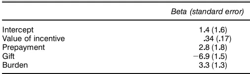
Table 1. Estimated Effects of Incentives on Response Rate (in Percentage Points) From Singer et al. (1999), Based on Their Meta-Analysis of Differences in Response Rates Between Smaller (or

Zero) and Larger Incentives Conditions Within Surveys

Beta (standard error)

NOTE: All coef’cients in the table are interactions with the “incentive” treatment. For exam-ple, the effect of an incentive ofxdollars is estimated to be 104%C036%xif the incentive is

postpaid, cash, and for a low-burden survey. The Consumer Price Index was used to adjust to 1999 dollars.

The regression model presented by the Singer et al. study includes incentive value, timing, form, and burden. The effects of mode, interaction between mode and incentive, and inter-action between burden and incentive were estimated and dis-regarded by Singer et al., because their effects were not sta-tistically signiŽcant. Table 1 summarizes their main result.

2.3 Reanalysis of Incentives Meta-Analysis Data

2.3.1 Motivation for the Reanalysis. We wanted to apply the results of the meta-analysis to the Social Indicators Survey (SIS), a telephone survey with a low burden (an interview that typically takes 45 minutes to an hour with no complications or follow-up). We wanted to decide whether to offer incentives and, if so, the timing, value, and form of the incentives. We were wary of directly using the model Žt by Singer et al. for several reasons:

¡ _{The intercept for the model is quite large, indicating a}

substantial effect for incentives even in the limit of $0 pay-outs. For preincentives, this is reasonable, because the act of contacting a potential respondent ahead of time might increase the probability of cooperation, even if the advance letter con-tained no incentive. For postincentives, however, we were sus-picious that a promise of a very small incentive would have much effect. The meta-analysis includes surveys with very low incentives, so this is not simply a problem of extrapolating beyond the range of the data. (The estimated intercept in the regression is not statistically signiŽcant; however, for the pur-pose of decision making, it cannot necessarily be ignored.)

¡ _{Under the model, the added effect for using a}

preincen-tive (rather than a postincenpreincen-tive) is a constant. It seems reason-able that this effect might increase with larger dollar payouts, which would correspond in the regression to an interaction of the timing variable with incentive value. Similarly, the model assumes a constant effect for switching from a low-burden to high-burden survey, but one might suspect once again that the difference between these two settings might affect the per-dollar beneŽt of incentives as well as the intercept. (In the context of Žtting a regression model from sparse data, it is quite reasonable to not try to Žt these interactions. For deci-sion making, however, it might not be the best idea to assume that these interactions are zero.)

¡ _{More generally, not all of the coefŽcient estimates in}

Table 1 seem believable. In particular, the estimated effect

for gift versus cash incentive is very large in the context of the other effects in the table. For example, from Table 1, the expected effect of a postpaid cash incentive of $10 in a

low-burden survey is 104C1040345ƒ609D ƒ201%, thus actually

lowering the response rate. It is reasonable to suspect that this reects differences between the studies in the meta-analysis, rather than such a large causal effect of incentive form.

¡ _{A slightly less important issue is that the regression}

model on the differencesz_i does not reect the hierarchical

structure of the data; the 62 differences are clustered in 39 sur-veys. In addition, it is not so easy in that regression model to account for the unequal sample sizes for the experimental con-ditions, which range from less than 100 to more than 2,000. A simple weighting proportional to sample size is not appro-priate, because the regression residuals include model error as well as binomial sampling error.

For the purpose of estimating the overall effects of incen-tives, the Singer et al. (1999) approach is quite reasonable and leads to conservative inferences for the regression parameters of interest. We set up a slightly more elaborate model because, for the purpose of estimating the costs and beneŽts in a par-ticular survey, we needed to estimate interactions in the model (e.g., the interaction between timing and value of incentive), even if these were not statistically signiŽcant.

2.3.2 Setting Up the Hierarchical Model. We thus decided to reŽt a regression model to the data used in the meta-analysis. When doing this, we also shifted over to a

hier-archical structure to directly model the 101 response ratesy_i

and thus handle the concerns at the end of the list in the pre-vious section. (As shown in DuMouchel and Harris 1983, a hierarchical model allows for the two levels of variation in a meta-analysis.)

We start with a binomial model relating the number of

respondents,ni, to the number of persons contacted,Ni (thus

yiDni=Ni), and the population response probabilitiesi:

ni¹bin4Ni1 i50 (1)

By using the binomial model, we are ignoring the ination of the variance due to the sampling designs, but this is a rela-tively minor factor here, because the surveys in this study had essentially one-stage designs.

The next stage is to model the probabilities, _i, in terms

of predictor variables, X. In general, it is advisable to use

a transformation before modeling these probabilities, because they are constrained to lie between 0 and 1. However, in our particular application area, response probabilities in telephone and face-to-face surveys are far enough from 0 and 1 that a linear model is acceptable:

i¹N44X‚5iCj4i51‘250 (2)

HereX‚is the linear predictor for conditioni,j4i5 is a

ran-dom effect for the survey jD11 : : : 139 (necessary in the

model because underlying response rates vary greatly), and‘

represents the lack of Žt of the linear model. We use the

nota-tionj4i5because the conditionsiare nested within surveysj.

Modeling (2) on the untransformed scale is not simply an approximation, but rather a choice to set up a more inter-pretable model. Switching to the logistic, for example, would

have no practical effect on our conclusions, but it would make all of the regression coefŽcients much more difŽcult to inter-pret.

We next specify prior distributions for the parameters in the

model. We model the survey-level random effectsj using a

normal distribution,

_j¹N401 ’2₅₀

(3)

There is no loss of generality in assuming a zero mean for the

_j’s if a constant term is included in the set of predictorsX.

Finally, we assign uniform prior distributions to the standard

deviation parameters‘ and’, p4‘ 1 ’5/1 (as in the

hierar-chical models of chap. 5 of Gelman, Carlin, Stern, and Rubin

1995) and to the regression coefŽcients‚. The parameters‘

and’ are estimated precisely enough (see the bottom rows of

Table 2) so that the inferences are not sensitive to the particu-lar choice of noninformative prior distribution. We discuss the

predictorsX in Sections 2.3.4 and 2.3.5.

2.3.3 Computation. Equations (1)–(3) can be combined to form a posterior distribution. For moderate and large

val-ues of N (such as are present in the meta-analysis data), we

can simplify the computation by replacing the binomial distri-bution (1) by a normal distridistri-bution for the observed response

rate y_iDn_i=N_i,

y_i¹approx_N4

i1 Vi51 (4)

whereViDyi41ƒyi5=Ni. (It would be possible to use the exact

binomial likelihood, but in our example this would just add complexity to the computations without having any effect on the inferences.) We can then combine this with (2) to yield

yi¹N44X‚5iCj4i51‘2CVi50 (5)

Boscardin and Gelman (1996) have discussed similar het-eroscedastic hierarchical linear regression models.

We obtain estimates and uncertainties for the parameters,

‚,‘, and ’ in our models using Bayesian posterior

simula-tion, working with the approximate model—the likelihood (5) and the prior distribution (3). For any particular choice of pre-dictive variables, this is a hierarchical linear regression with

two variance parameters,‘ and’.

Given‘ and ’, we can easily compute the posterior

dis-tribution of the linear parameters, which we write as the vec-tor ƒ D4‚1 5. The computation is a simple linear

regres-sion of yü on Xü with variance matrix èü, where W is the

101€39 indicator matrix mapping conditions i to surveys

j4i5, y is the vector of response rates, 4y₁1 : : : 1 y₁₀₁5,yü the

vector of length 140 represented by y followed by 39 0s,

XüD

ear regression computation gives an estimate ƒO and

vari-ance matrix Vƒ, and the conditional posterior distribution

is ƒ—‘ 1 ’ 1 X1 y_¹ N4ƒ1 VO ƒ5 (see, e.g., Gelman et al. 1995, chap. 8).

The variance parameters‘ and’ are not known, however,

thus we compute their joint posterior density numerically on

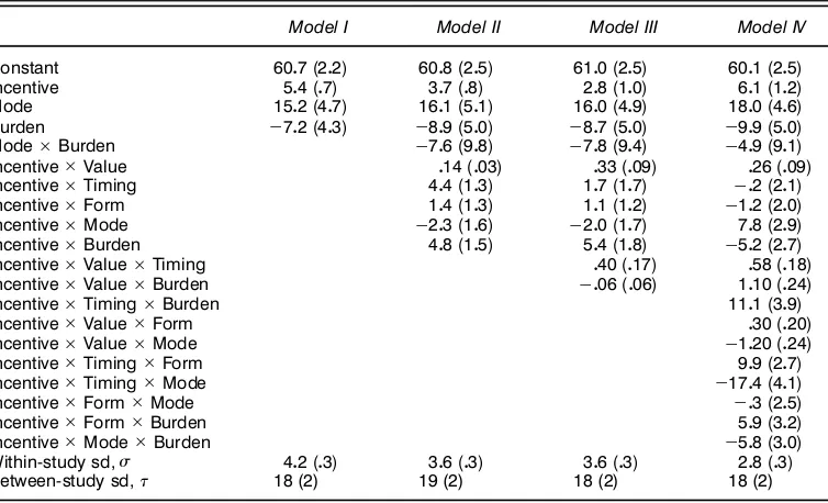
Table 2. Estimated Coef’cients From the Hierarchical Regression Models Fit to the Meta-Analysis Data, With Half-Interquartile Ranges in Parentheses, Thus Giving Implicit 50% Intervals

Model I Model II Model III Model IV

Constant 6007(202) 6008(205) 6100(205) 6001(205)

NOTE: Numbers are to be read as percentage points. All coef’cients are rounded to one decimal point, except for those including Value, which are given an extra signi’cant digit because incentive values are commonly in the tens of dollars. Model III is our preferred model, but we also perform decision calculations under model II, because it is comparable with the no-interactions model ’t by Singer et al. (1999).

a two-dimensional grid. The marginal posterior density of the variance parameters can be computed using the formula

p4‘ 1 ’—X1 y5

The foregoing equation holds for any value ofƒ; for

compu-tational simplicity and stability, we chooseƒD Oƒ (recall that

O

ƒ implicitly depends on‘ and’) to obtain

p4‘ 1 ’—X1 y5/ —V_ƒ—1=2_—è

Once the posterior distribution grid for‘ and ’ has been

computed and normalized, we draw 11000 values of‘ from

the grid. For each‘, we draw a corresponding’. To do this,

we condition on each‘ and use the normalized column

cor-responding to it as the marginal distribution from which we

draw’. We sampled from a 21€21 grid, set up to contain the

bulk of the posterior distribution (as in Gelman et al. 1995, chap. 3). Repeating the computations on a Žner grid did not change the results.

For each of the 1,000 draws of 4‘ 1 ’5, we draw ƒ D

4‚1 5 from the normal distribution with mean ƒO and

vari-ance matrixVƒ. We use the median and quantiles of the 11000

values ofƒ to summarize parameter estimates and

uncertain-ties, focusing on the inferences for‚(i.e., the Žrst several

ele-ments ofƒ, corresponding to the regression predictors). These

1,000 draws are enough that the estimates are stable.

2.3.4 Potential Predictor Variables. To construct the

matrixX of predictors, we considered the following

explana-tory variables and their interactions:

1. Incentive: An indicator for whether an incentive was used in this condition of the survey

2. Value: Dollar value of the incentive, deŽned only if

IncentiveD1

3. Timing: ƒ1=2 if given after the survey, 1/2 if given

before, deŽned only if IncentiveD1

4. Form:ƒ1=2 if gift, 1/2 if cash, deŽned only ifIncentive

D1

5. Mode:ƒ1=2 if telephone, 1/2 if face-to-face

6. Burden: ƒ1=2 if low, 1/2 if high.

These last Žve variables are those listed near the beginning of Section 2.2.

We have arranged the signs of the variables so that, from prior knowledge, one might expect the coefŽcients interacted with incentive to be positive. We code several of the binary

variables as ƒ1=2 or 1=2 (rather than the traditional coding

of 0 and 1) to get a cleaner interpretation of various nested main effects and interactions in the model. For example, the coefŽcient for Incentive is now interpreted as averaging over the two conditions for Timing, Form, Mode, and Burden. The

coefŽcient for Incentive€Timing is interpreted as the

addi-tional effect of Incentive if administered before rather than after the survey.

Because of the restrictions (i.e., Value, Timing, and Form

are only deŽned if IncentiveD1), there 35 possible regression

predictors, including the constant term and working up to the

interaction of all 6 factors. The number of predictors would, of course, increase if we allowed for nonlinear functions of incentive value.

Of the predictors, we are particularly interested in those that include interactions with I, the Incentive indicator, because these indicate treatment effects. The two-way interactions in the model that include I can thus be viewed as main effects of the treatment, the three-way interactions can be viewed as two-way interactions of the treatment, and so forth.

2.3.5 Setting Up a Series of Candidate Models. We Žt a series of models, starting with the simplest and then adding interactions until we pass the point at which the existing data could estimate them effectively, then Žnally choosing a model that includes the key interactions needed for our deci-sion analysis. For each model, Table 2 displays the vector of coefŽcients, with uncertainties (half-interquartile ranges) in parentheses. The bottom of the table displays the estimated components of variation. The within-study standard deviation

‘ is around 3 or 4 percentage points, indicating the accuracy

with which differential response rates can be predicted within

any survey; the between-study standard deviation’ is around

18 percentage points, indicating that the overall response rates vary greatly, even after accounting for the survey-level predic-tors (Mode and Burden).

Model I includes main effects only and is included just as a comparison with the later models. Model I is not substan-tively interesting, because it includes no Incentive interactions and thus Žts the effect of incentives as constant across all con-ditions and all dollar values.

Model II is a basic model with 10 predictors: the constant term, the 3 main effects, and the 6 two-way interactions. This model is similar to those Žt by Singer et al. (1999) in that the added effects per dollar of incentive are constant across all conditions.

Model III brings in the three-way interactions that include

Incentive€Value interacting with Timing and Burden, which

allow the per-dollar effects of incentives to vary with the con-ditions that seem most relevant to our study. The here differ quite a bit from the previous model (and from that of Singer et al.), with different slopes for different incentive conditions.

SpeciŽcally, the positive Incentive€ Value € Timing

inter-action implies that prepaid incentives have a higher effect per dollar compared to postpaying.

Model IV includes the main effects and all two-way and three-way interactions. We decided to discard this model, because it yielded results that did not make sense, most notably negative per-dollar effects of incentives under many

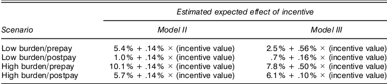
Table 3. Summary of Two Models Fit to the Meta-Analysis Data Assuming Telephone Surveys With Cash Incentives

Estimated expected effect of incentive

Scenario Model II Model III

Low burden/prepay 5.4 % + .14 %€(incentive value) 2.5 % + .56 %€(incentive value) Low burden/postpay 1.0 % + .14 %€(incentive value) .7 % + .16 %€(incentive value) High burden/prepay 10.1 % + .14 %€(incentive value) 7.8 % + .50 %€(incentive value) High burden/postpay 5.7 % + .14 %€(incentive value) 6.1 % + .10 %€(incentive value)

NOTE: Estimated effects are given as a function of the dollar value of the incentive.

conditions (as indicated by negative interactions containing Incentive and Value). Also, adding these hard-to-interpret interactions increased the uncertainties of the main effects and lower-level interactions in the model. We thus retreated to model III.

2.3.6 Summary of the Fitted Models. To recapitulate, the ideal model for the effects of incentives would include interac-tions at all levels. Because of data limitainterac-tions, it is not possible to accurately estimate all of these interactions, and so we set up a restricted model (model III) that allows the most impor-tant interactions and is still reasonable. In our cost-beneŽt analyses, we work with model II (because it is similar to the analysis of Singer et al.) and model III (which includes inter-actions that we consider important). Table 3 summarizes the estimated effects of incentives under the two models.

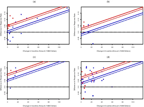
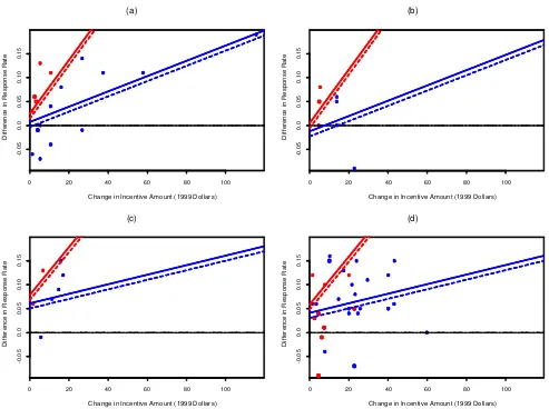
To understand the models better, we display the estimates of the effect of incentive versus dollar value of incentive in Figures 1 and 2. A main effect of Incentive is an intercept on such a graph, with the slope corresponding to the coefŽcient

for Incentive€Value. Two-way interactions of Incentive with

the categorical predictors Timing, Form, Mode, and Burden show up as shifts in the intercepts, and three-way interactions

of Incentive€Value with the predictors Timing, Form, Mode,

and Burden appear as unequal slopes in the lines.

We display each model as four graphs corresponding to the two possible values of the Burden and Mode variables. Within each graph, we display lines for the prepay condition in red and postpay in blue, with solid and dashed lines for the cash and gift conditions. This allows us to display 16 lines, which correspond to all combinations of the 4 binary predictors Tim-ing, Form, Mode, and Burden as they interact with Incentive

(the intercepts) and with Incentive€Value (the slopes). These

plots thus allow us to display the model in all its potential complexity, even up to six-way interactions. (The plots do not

display the main effects of Mode, Burden, or Mode €

Bur-den, but this is not a problem, because in our study we are interested only in the effects of incentives.)

We complete the graphs by including a dotted line at 0 (the comparison case of no incentive) and displaying on each graph

the difference dataziused in the Singer et al. (1999) regression

on the y-axis and the difference in incentives on the x-axis.

Red and blue dots indicate prepaid and postpaid incentives, with the points put into the appropriate subgraphs correspond-ing to the mode and burden of their surveys. It is clear from these graphs that incentives generally have positive effects, and that prepaid incentives tend to be smaller in dollar value.

(c)

Change in Incentive Amount (1999 Dollars)

D

Change in Incentive Amount (1999 Dollars)

D

Change in Incentive Amount (1999 Dollars)

D

Change in Incentive Amount (1999 Dollars)

D

Figure 1. Estimated Increase (posterior mean) in Response Rate Versus Dollar Value of Incentive for Model II. Separate plots show estimates for (a) low-burden, telephone survey; (b) low-burden, face-to-face survey; (c) high-burden, telephone survey; and (d) high-burden, face-to-face survey. For application to the SIS, we focus on the upper-left plot. The red and blue lines indicate estimates for prepaid and postpaid incentives, respectively. The solid lines and solid circles represent cash incentives. Dotted lines and open circles represent gift incentives. Finally, the red and blue dots show observed change in response rate versus change in incentive value for prepaid and postpaid incentives.

To summarize, all of the lines in Figure 1 (corresponding to model II) are parallel, which implies that in this model the additional effect per dollar of incentive is a constant (from Table 3, an increase of .14 percentage points in response rate). The blue lines are higher than the red lines, indicating that prepaid incentives are more effective, and the solid lines are higher than the dotted lines, indicating that cash is estimated to be more effective than gifts of the equivalent value. The different positions of the lines in the four graphs indicate how the estimated effects of incentives vary among the different scenarios of burden and mode of survey.

Similarly, the lines in Figure 2 show the estimated effects for model III. The red lines are steeper than the blue lines, indicating higher per-dollar effects for prepaid incentives. The red lines are also entirely higher than the blue (i.e., the lines do not cross), indicating that prepaid incentives are estimated to be higher for all values, which makes sense. The other patterns in the graphs are similar to those in Figure 1, implying that the other aspects of model III are similar to those of model II. To check the Žts, we display in Figure 3 residual plots of

prediction errors for the individual data points y_i, showing

telephone and face-to-face surveys separately and, as with the previous plots, using colors and symbols to distinguish

tim-ing and form of incentives. There are no patterns indicattim-ing problems with the basic Žt of the model.

Another potential concern is the sensitivity of model Žt to extreme points, especially because we have no particular

rea-son to believe the linearity of the Incentive € Value effect.

In particular, in Figure 3(a), corresponding to low burden and phone, the survey indicated by the solid blue dot on the upper right is somewhat of an outlier. ReŽtting the model without this survey gave us very similar results (e.g., the Žrst model in

Table 3 changed from 504%C014%x to 509%C012%x), and

so we were not bothered by keeping it in the model.

3. APPLICATION TO THE SOCIAL INDICATORS SURVEY

We now apply our inferences from the meta-analysis to the SIS, a telephone survey of New York City families (GarŽnkel and Meyers 1999). The survey was divided into two strata: an individual survey, which targeted all families (including single adults and couples), and a caregiver survey, which was restricted to families with children. Our recommendations for these two strata are potentially different because in the caregiver survey, more than half of the interviews are stopped

Change in Incentive Amount (1999 Dollars)

Change in Incentive Amount (1999 Dollars)

D

Change in Incentive Amount (1999 Dollars)

D

Change in Incentive Amount (1999 Dollars)

D

Figure 2. Estimated Increase (posterior mean) in Response Rate Versus Dollar Value of Incentive for Model III. Separate plots show estimates for (a) low-burden, telephone survey; (b) low-burden, face-to-face survey; (c) high-burden, telephone survey; and (d) high-burden, face-to-face survey. For application to the SIS, we focus on (a). The red and blue lines indicate estimates for prepaid and postpaid incentives, respectively. The solid lines and solid circles represent cash incentives. Dotted lines and open circles represent gift incentives. Finally, the red and blue dots show observed change in response rate versus change in incentive value for prepaid and postpaid incentives.

Predicted response rate

O

Predicted response rate

O

Figure 3. Residuals of Response Rate Meta-Analysis Data Compared With Predicted Values from Model III. Residuals for (a) telephone and (b) face-to-face surveys are shown separately. As in the previous ’gures, red and blue dots indicate surveys with prepaid and postpaid incentives, and the solid and open circles represent cash and gift incentives.

immediately because there are no children at the sampled tele-phone number (as is apparent in the Žrst column of Table 6). This makes a preincentive less desirable for the caregiver sur-vey, because most of the payments mailed out before the tele-phone call would be wasted.

Section 3.1 details our method for estimating the impact of incentives on the telephone survey, Žrst for postpaid incentives and then for prepaid, which are slightly more complicated because of the difŽculty of reaching telephone households by mail. We integrate these estimates into a cost-beneŽt analysis in Section 3.2.

3.1 Estimated Costs and Cost Savings With Incentives

We assume that the target number of respondents is Žxed. When a Žnancial incentive is used, the (expected) response rate goes up, and fewer calls need to be made to obtain the same number of interviews. Incentives, therefore, can reduce the amount of time that interviewers spend on the phone, thus saving money that might make up for part or all of the cost of the incentive.

How much money is saved when fewer calls are made? To answer this question, Žrst we need to know the approximate cost of each call. We do not know this value, but Schulman, Ronca, Bucuvalas, Inc. (SRBI) did give us enough informa-tion to determine the length of time spent on each noninter-view. We calculated these values by taking the time that each interview was completed and comparing it with the time that this interviewer completed the previous interview. (The Žrst interview of the day for each interviewer was dropped from the analysis.) Of course, we did not believe that interviewers were on the phone every second between interviews; we did believe, however, that the cost for the principals was approx-imately the same whether the interviewer was productive or not.

We had data available on a total of 109,739 phone calls, of which 2,221 were complete interviews. Interviewers spent a total of 271,035 minutes on these calls, of which 68,936 minutes were spent on completed interviews. The average length of time spent on a call, therefore,

was 2711035=1091739D2047 minutes; excluding completed

interviews, the time per call is reduced to 42711035ƒ

6819365=41091739ƒ212215D1088 minutes.

We then made a rough estimate of the cost of interviewing, which came to $24.80 per hour (see Table 4). The

approx-imate cost of a non-interview call, therefore, was $24080€

41088=605D$078.

Finally, we categorized all phone numbers into the follow-ing status codes:

¡ Nonhousehold: it was discovered that the telephone

num-ber belonged to a business or other nonhousehold

¡ Not screened: no one ever answered

¡ Not eligible: it was determined that there were no children

in the household (for the caregiver survey), or there were no adults in the household, or no one in the household was a U.S. citizen

¡ Incapable: hearing problem or too sick to participate

Table 4. Estimated Costs per Hour of Telephone Interviewing for the SIS

Expense Estimated cost per hour

Interviewer hourly wage $10000

Interviewer FICA and unemployment, etc. 1050

Cost of phone calls, at 10 cents per minute 6000

Supervisors, 1 per 10 interviewers 2000

Supervisor FICA and unemployment, etc. 030

Miscellaneous overhead 5000

Total $24080

¡ Language barrier: no one in the household spoke English

or Spanish

¡ Refusals: the designated respondent refused to participate

in the survey

¡ Noninterviews: the interviewers gave up trying to contact

the respondent after numerous attempts

¡ Incompletes: an interview was started but not completed

¡ Completed interviews.

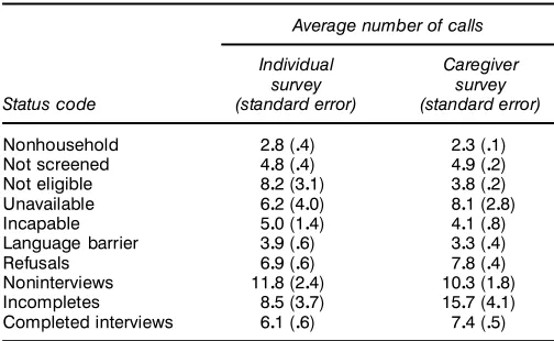
Table 5 gives the average number of calls made per tele-phone number, categorized based on the Žnal status codes; these averages range from 2 or 3 for nonhousehold telephone numbers to more than 10 for noninterviews. The averages are given with standard errors (computed as the standard devia-tion of the number of calls, divided by the square root of the number of telephone numbers in the category). Inspection of the rows of the table reveals that the average numbers of calls per telephone number for the individual and caregiver surveys are statistically indistinguishable for all categories except “not eligible.” This makes sense because the only substantial dif-ference in the surveys is their eligibility criteria.

We estimate the amount saved through the use of Žnancial incentives by projecting how the incentive would change the number of calls in each of the various status codes. Given our estimate of the positive effect of incentives, this would reduce the number of calls made, which would in turn reduce the

Table 5. Average Number of Interviewer Calls per Telephone Number, Classi’ed by Status Code, for the SIS Individual and Caregiver Surveys

Average number of calls

Individual Caregiver

survey survey

Status code (standard error) (standard error)

Nonhousehold 208(04) 203(01)

NOTE: Each entry is an average (with standard error in parentheses). The averages are used to estimate the number of telephone calls saved in counterfactual scenarios in which fewer telephone numbers need to be called. The two surveys are statistically signi’cantly different in only one category, “not eligible,” which makes sense given that the major difference between the individual and caregiver surveys is in the eligibility rules.

cost of the survey as a whole. We assume that incentives will affect the number of calls of each status (as illustrated in detail in Sec. 3.1.1) but not the number of calls required to reach someone in a given status code. This assumption is reasonable because the largest effect of incentives should be to inspire nonresponders to respond, not to make them easier to reach.

To estimate the number of phone calls required under incen-tives, we reason that for a Žxed number of completed inter-views, the required list of phone numbers is inversely propor-tional to the response rate when all else is considered equal. For example, assume that a survey with a 50% response rate required 12,000 phone numbers to obtain 1,000 completed interviews. If the response rate were to increase to 60%, then one could assume (if all else was held constant) that one would

need only 121000=4060=0505D101000 numbers for the same

1,000 interviews. Therefore, increasing the response rate by 10% would require 2,000 fewer numbers.

In practice, the computations become more complicated, because the number of calls required would decrease more for some status codes than for others. SpeciŽcally, the number of refusals, noninterviews and incompletes would decline much more quickly as the response rate increases, compared with other status codes. If the response rate were to increase from 50% to 60%, for example, and the number of completed inter-views were kept constant at 1,000, then the number of refusals, noninterviews and incompletes would decline (in total) from 1,000 to 667, a 33% decrease, whereas other noninterview codes would decline by 17%. This could have an effect on the total number of calls needed and thus could affect the calcu-lation of savings.

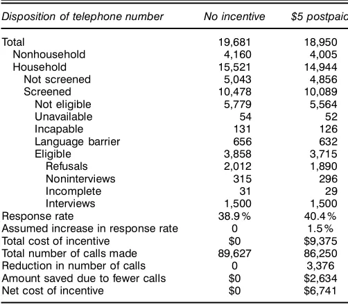
3.1.1 Postpaid Incentives. Table 6 illustrates the compu-tations for a $5 postincentive for the caregiver survey, using the increase in response rate estimated from model III. The “no incentive” column of the table gives the actual results

Table 6. Disposition of Telephone Numbers for the Caregiver Survey and the Expected Scenario for a $5 Postpaid Incentive

Disposition of telephone number No incentive $5 postpaid

Total 19,681 18,950

Response rate 38.9 % 40.4 % Assumed increase in response rate 0 1.5 % Total cost of incentive $0 $9,375 Total number of calls made 89,627 86,250 Reduction in number of calls 0 3,376 Amount saved due to fewer calls $0 $2,634 Net cost of incentive $0 $6,741

NOTE: For the incentive scenario, the increase in response rate is computed based on model III (see Table 3) for a low-burden telephone survey with postpaid incentives, and the other numbers are then determined based on the assumption that the number of completed inter-views is ’xed.

from the SRBI survey, and the other column is Žlled in using modeling assumptions:

1. We start near the bottom of the table, at the row labeled “Assumed increase in response rate.” The value of 1.5% here is the expected increase from model III as given in Table 3 for a low-burden telephone survey with a $5 postpaid incentive.

2. The expected increase of 1.5% added to the observed

response rate of 11500=31858D3809% in the no-incentive case

yields an expected response rate of 40.4% with a $5 postpaid incentive.

3. The number of interviews is held Žxed (in this case, at 1,500), and so the expected number of eligible households

required is backcalculated to be 11500=4004%D31715.

4. The sum of Refusals, Noninterviews, and Incompletes is

then reduced from 31858ƒ11500D21358 to 31715ƒ11500D

21215: the number of eligible households minus the number of

completed interviews. We assume that the three categories are reduced by equal proportions compared with the “no incen-tive” case.

In order to evaluate the importance of this assump-tion, we consider the sensitivity of our conclusions to vari-ous alternatives. One possible alternative assumption is that the incentive decreases the rate of Refusals but has no effect on the rates of Noninterviews and Incompletes. For example, in Table 6, this would mean that the number of Noninter-views and Incompletes under the incentive condition become

315431715=318585D303 and 31431715=318585D31, and the

number of Refusals then drops to 31715ƒ303ƒ31D11882.

Conversely, we can assume the other extreme—that the rate of

Refusals is unchanged, and thus 21012431715=318585D11937,

with the remaining decrease in the number of households attributed to fewer Noninterviews and Incompletes.

Under each of the two extreme assumptions, we recom-pute the reduction in expected total calls (again using the aver-ages of calls per code from Table 5). This propagates to the expected net cost of incentives; in the example of Table 6, this changes from $6,741 to $6,761 under the Žrst assumption (more Noninterviews and Incompletes, which requires more calls) or $6,630 under the second assumption (more Refusals, which requires relatively few calls). Either way, this is less than a 2% change in costs. We found similar results for the other scenarios and concluded that our total cost estimates and decision analyses were not sensitive to our assumptions about the dispositions of these calls.

5. The phone calls that do not lead to eligible households (Nonhousehold, Not screened, Not eligible, Unavailable, Inca-pable, and Language barrier) are all decreased in proportion to the number of eligible households required. That is, in Table 6 they are all multiplied by 3,715/3,858. The assumption of pro-portionality is reasonable here, because we would expect the incentive to affect only people being interviewed; it would not affect (or would affect only very slightly) nonhousehold tele-phone numbers, ineligible households, and others.

6. We have completed calculating the expected number of phone calls of each type required to complete 1,500 interviews under the assumed effectiveness of the incentive. We now adjust the lower part of Table 6 to estimate costs. First, the total cost of incentives is computed as the cost per incentive

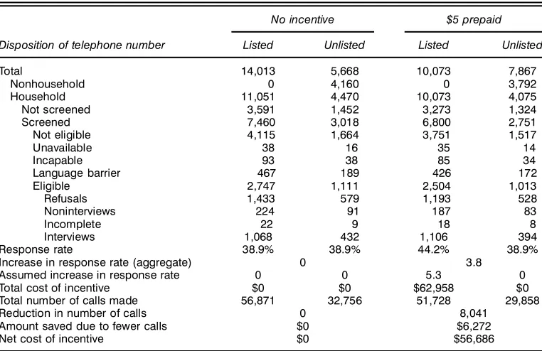
Table 7. Disposition of Telephone Numbers for the Caregiver Survey and the Expected Scenario for a $5 Prepaid Incentive

No incentive $5 prepaid

Disposition of telephone number Listed Unlisted Listed Unlisted

Total 14,013 5,668 10,073 7,867

Nonhousehold 0 4,160 0 3,792

Household 11,051 4,470 10,073 4,075

Not screened 3,591 1,452 3,273 1,324

Screened 7,460 3,018 6,800 2,751

Not eligible 4,115 1,664 3,751 1,517

Unavailable 38 16 35 14

Incapable 93 38 85 34

Language barrier 467 189 426 172

Eligible 2,747 1,111 2,504 1,013

Refusals 1,433 579 1,193 528

Noninterviews 224 91 187 83

Incomplete 22 9 18 8

Interviews 1,068 432 1,106 394

Response rate 38.9% 38.9% 44.2% 38.9%

Increase in response rate (aggregate) 0 3.8 Assumed increase in response rate 0 0 5.3 0 Total cost of incentive $0 $0 $62,958 $0 Total number of calls made 56,871 32,756 51,728 29,858

Reduction in number of calls 0 8,041

Amount saved due to fewer calls $0 $6,272

Net cost of incentive $0 $56,686

NOTE: Compare with Table 6. The divisions into listed and unlisted phone numbers are based on the assumption that 28.8% of all residential telephone numbers in all categories are unlisted and given the knowledge that listed business numbers were already screened out of the survey.

(adding $1.25 per incentive to account for mailing and admin-istrative costs), multiplied by the number of interviews. In this

case, this is 11500€$6025D$91375. (Costs would be lower

under the assumption that incentives are given just for refusal conversion.)

7. The total number of calls is computed by multiplying the number of calls in each status code by the average number of calls per code in Table 5.

8. The estimated amount saved due to fewer calls is com-puted as the reduction in number of calls multiplied by $.78, which is our estimate of the average cost of a noninterview call.

9. The net cost of incentives is the total cost minus the esti-mated amount saved due to fewer calls. Because the incentive reduces the total number of calls required, this net cost is less than the direct dollar cost of the incentives (in Table 6, the estimated total and net costs are $9,375 and $6,741).

3.1.2 Prepaid Incentives. The analysis of preincentives was conducted in much the same fashion as for postincen-tives. One difference is that incentives are sent to all res-idential households that can be located through a reverse directory. We assume that phone numbers are generated ran-domly, as with any other survey, with known business num-bers excluded from the start. A reverse directory is then used to Žnd the address for each residential number. Some of these numbers would be unlisted, of course, and thus their addresses would be unknown. According to Survey Sampling, Inc.(http://www.worldopinion.com/), the unlisted rate for the New York metropolitan area is 28.8%, so approximately 70% of all households would receive the preincentive and 30% would not.

The effect of the incentive is thus reduced in proportion to the unlisted rate. This is the case because preincentives would be sent, and thus would improve the response rate, only among households with listed phone numbers. The response rate would therefore have to be computed separately for both listed and unlisted contacts.

The computations are illustrated in Table 7 for a $5 prepaid incentive. Response rates are calculated separately for listed and unlisted numbers, and the total cost of preincentives is equal to the number of listed households.

3.2 Cost-Bene’t Analysis

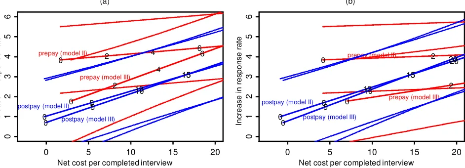
Figure 4 displays the net expected increase in response rate, plotted against the estimated net cost per respondent of incen-tives for the SIS, for the individual and caregiver studies. Esti-mates are given based on two different models obtained from the meta-analysis, models II and III (see Table 3). As always, prepaid incentives are shown in red; postpaid, in blue.

(Dot-ted lines on the graph show 1 standard error bounds derived

from the posterior uncertainties in the expected increase in response rate from the Bayesian meta-analysis.) The expected increase in response rate is a linear function of estimated net costs, which makes sense because the models Žt in Section 2 are all linear, as are the cost calculations described in Section 3.1. The numbers on the lines indicate incentive payments. At zero incentive payments, estimated effects and costs are nonzero, because the models in Table 3 have nonzero inter-cepts (corresponding to the effect of making any contact at all) and also we are assuming a $1.25 processing cost per incen-tive. In general, the prepaid incentives cost much more per completed interview because they are sent to nonrespondents as well as respondents.

Net cost per completed interview

Net cost per completed interview

In

postpay (model III)

0 prepay (model II) 2

postpay (model III)

Figure 4. Expected Increase in Response Rate Versus Net Cost of Incentive per Respondent, for Prepaid and Postpaid Incentives, for the (a) Individual and (b) Caregiver Surveys. On each plot, the two lines of each color correspond to the two models in Table 3 (with dotted lines showing 1 standard error bounds). The numbers on the lines indicate incentive payments. At zero incentive payments, estimated effects and costs are nonzero, because the models have nonzero intercepts (corresponding to the effect of making any contact at all) and we also are assuming a $1.25 processing cost per incentive.

Based on this analysis, we Žnd prepayment to be slightly more cost-effective for the survey of individuals, with the case less clear for the caregivers survey.

The costs and response rates we have calculated are expec-tations, in the sense that the effect sizes estimated from the meta-analysis can be interpreted as an average over the population of surveys represented in the study. Sec-ond, even if the effect of incentives for this particular sur-vey or class of sursur-veys were known, the actual response rate would be uncertain; for example, a response rate of

11500=31858D39% has an inherent sampling standard

devia-tion ofp03941ƒ0395=31858D08%.

In the range of costs and response rates considered here, it is reasonable to suppose utility to be linear in both costs and response rates. Thus it makes sense to focus on the expected

values, with the 1 standard error bounds giving a sense of

the uncertainty in the actual gains to be expected from the incentives.

4. DISCUSSION

4.1 Comments on the Meta-Analysis

We are not completely satisŽed with our meta-analysis, but we believe it to be a reasonable approach to the problem given the statistical tools currently available. To review, our two key difŽculties are (1) the data are sparse, with only 101 exper-imental conditions available to estimate potentially six levels of interactions that combine to form 35 possible linear predic-tors (see Sec. 2.3.4), and (2) the only consistently randomized factor in the experiments is the incentive indicator itself; the other factors are either observational (burden, mode) or exper-imental but generally not assigned randomly (value, timing, form). This is a common problem when a meta-analysis is used to estimate a “response surface” rather than simply an average effect (see Rubin 1989). A third potential difŽculty arises from the clustering in the data (between two and Žve

observations for each experiment), but this was easily handled using a hierarchical model as discussed in Section 2.3.2.

Because of the sparseness in the data, many coefŽcients of interest in the model have large standard errors. Because of the nonrandomized design (which is unavoidable because the 39 different studies were conducted at different times with different goals), coefŽcient estimates cannot automatically be given direct causal interpretations, even if they are statistically

signiŽcant. For example, the estimated effect of ƒ609% in

response rate for a gift (compared with the equivalent incen-tive in cash) in the Singer et al. (1999) analysis (see Table 1) is presumably an artifact of interactions in the data between the form of the incentive and other variables that affect response rates. To put it most simply, the surveys in which gifts were used may be surveys in which, for some other reasons, incen-tives were less effective.

We dealt with both design difŽculties taking the following approach:

¡ _{Parameterize the variables (as illustrated in Sec. 2.3.4)}

so that when higher-level interactions are included in the model, main effects and low-level interactions still retain their interpretations as average effects.

¡ _{Include all main effects and interactions that are}

expected to be important or are of primary interest in the

sub-sequent decision analysis, for example, Incentive€Value €

Form.

¡ _{As is standard in the analysis of variance, proceed in a}

nested fashion, starting with main effects and adding interac-tions. Whenever an interaction is included, all of its associated main effects are already also included (with the exception of variables, such as Timing, that are deŽned only when inter-acted with Incentive).

As discussed in Section 2, high levels of interactions are a modeling necessity, not merely a theoretical possibility: for example, differing marginal effects for incentives for different conditions (e.g., low vs. high burden, prepaid vs. postpaid)

correspond to three-level interactions at the very least. And we have not even considered nonlinear effects of the dollar values of incentives. Perhaps surprisingly, the linear model appears to Žt reasonably well for high incentive values, but less well so near 0.

The steps of our informal Bayesian strategy seem reason-able, but they obviously cannot represent anything close to an optimal mode of inference. We would feel more comfort-able with a hierarchical model that includes all interactions in the model, controlling the parameter estimates using shrink-age rather than by setting estimates to 0 (Gelman et al., 1995, chap. 13). However, this strategy requires further research into setting up a reasonable class of prior distributions.

A related approach is the formal selection of subsets of pre-dictors using Bayesian methods (see, e.g., George and McCul-loch 1993; Madigan and Raftery 1994; Draper 1995), but we doubt that these methods are appropriate for our problems, because formal Bayesian selection rules tend to select rela-tively few predictors, which in this case could lead to a model

that does not allow interactions such as Incentive€Value €

Timing that are important in the subsequent decision analysis. Of course, such information could be included in the form of inequality constraints or informative prior distributions, and this moves us toward the sorts of models that we would like to Žt. In the meantime, however, we believe that useful decision analyses can be made using less formal methods of model building.

4.2 Recommendations for Survey Incentives

So, now that we have done our analysis, what action do we recommend? For both the individual and caregiver surveys, small incentives appear reasonable, but Figure 4 implies that one should expect to pay more than $20 per completed inter-view to get even a 5% increase in response rate. Our estimates for the overall effects of incentives are fairly small, which makes sense given the range of observed differences in the data (see Fig. 1 or Fig. 2).

Postpaid incentives would be more effective if they were given as refusal conversions rather than to all of the intervie-wees. For the caregivers survey, even small preincentives can become very expensive, because they must be mailed to all of the persons screened out in the interviews. In any case, we would give a cash incentive, because this is easier than a gift and evidence suggests that gifts are less effective than equiv-alent amounts of cash. In other settings it may make sense to consider gifts as an option, for example, if the gifts are donated by some outside organization, or if it is feasible to give items such as coupons, price discounts, or rafe tickets that cost less than their nominal value. It is easy to estimate the effects of such strategies by simply altering the estimated costs (as in Table 6) appropriately.

One strategy that is not addressed by the meta-analysis is the combination of preincentives and postincentives. A sim-ple analysis would assume additivity, but perhaps the combi-nation of the two forms of incentives would work better (or worse) than the sum of their individual effects. Because of the screening of respondents (two-thirds of our total sample size

Callback number

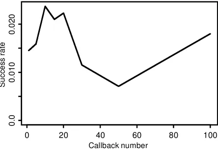
Figure 5. Proportion of Calls That Resulted in a Completed Inter-view for the Caregiver Portion of the SIS, as a Function of the Callback Number. The ’rst point on the graph indicates initial calls; the later points correspond to calls 2–5, 6–10, 11–15,: : :, 51–100. The proba-bility of a completed interview is close to 1.5% for all callbacks, indicat-ing that SRBI is ef’ciently allocatindicat-ing its resources in decidindicat-ing how long to follow up with callbacks. A total of 54% of the completed interviews required more than 3 callbacks, 12% required more than 15 calls, and 3% required more than 50 calls.

of 2,250 is allocated to the caregivers), we do not recommend presending letters or incentives in our survey.

Incentives should also be considered in the total context of survey costs. For example, an effective strategy for increas-ing response rate in the SIS was to monitor the interviewer-speciŽc response rates and then allocate more phone time to the more effective interviewers. The marginal gains from additional callbacks (Triplett 1997) can also be considered. In our survey, callbacks at all stages had an approximately 1.5% chance of resulting in a completed interview (see Fig. 5). The expected marginal costs of getting an interview can then be compared using three strategies: (1) getting a fresh phone number, (2) conducting more intensive callbacks, and (3) pay-ing an incentive.

Singer et al. (1999) and Singer (2001) discussed various other issues of the implementation and effects of incentives, and Cantor and Cunningham (1999) provided advice on a range of strategies for contacting telephone respondents. Our analysis is not intended to be a substitute for these practi-cal recommendations. Rather, in applying research Žndings to a new telephone survey, we have attempted to explicitly lay out the costs and beneŽts of proposed strategies, such as incentives, in the context of the particular survey. This is in line with the general recommendations of decision analysis (see, e.g., Clemen 1996) that the key step is to enumerate deci-sion alternatives and consider their expected consequences. We found this perspective to have implications in setting up regression models whose parameter estimates were used as input for the decision analysis and also in the explicit account-ing calculations illustrated in Tables 6 and 7.

4.3 Regression Modeling for Decision Analysis

We conclude with some recommendations for applying regressions—or, more generally, inferences from any statisti-cal models—to cost-beneŽt statisti-calculations. First, if a particular

factor is involved in the decision, then it should be included in the model. For example, we had to choose between pre-incentives and postpre-incentives, and so the model had to allow for interaction between timing and value of incentives, even if the estimate of that interaction is statistically insigniŽcant. Second, it is important that the Žnal model chosen make sense, and this judgment can perhaps best be made graphically, as in Figures 1 and 2. Third, the cost structure of the applica-tion should be carefully laid out. We spent quite a bit of effort doing that in Section 3 to emphasize the detail work that must be done for an inference to be used in a cost-beneŽt analysis.

ACKNOWLEDGMENTS

This research was suggested by Professor Marcia Meyers, School of Social Work, University of Washington, Seattle. We thank Kevin Brancato and Hailin Lou for research assis-tance, Phillip Price, T. E. Raghunathan, Bob Shapiro, Julien Teitler, and several referees for helpful comments, and the U.S. National Science Foundation for support through grants SBR-9708424, SES-99-87748, and Young Investigator Award DMS-9796129. We especially thank Eleanor Singer and John Van Hoewyk for generously sharing with us the data from their meta-analysis, and SRBI (Schulman, Ronca, Bucuvalas, Inc.) for sharing with us the data on the disposition of telephone calls in the 1997 Social Indicators Survey.

[Received February 2001. Revised September 2002.]

REFERENCES

Boscardin, W. J., and Gelman, A. (1996), “Bayesian Regression With Para-metric Models for Heteroscedasticity,” Advances in Econometrics, 11, A87–109.

Cantor, D., and Cunningham, P. (1999), “Methods for Obtaining High Response Rates in Telephone Surveys,” paper presented at the Workshop on Data Collection for Low-Income Populations, Washington, D.C. Clemen, R. T. (1996),Making Hard Decisions(2nd ed.), PaciŽc Grove, CA:

Duxbury.

Draper, D. (1995), “Assessment and Propagation of Model Uncertainty” (with discussion),Journal of the Royal Statistical Society, Ser. B, 57, 45–97. DuMouchel, W. M., and Harris, J. E. (1983), “Bayes Methods for Combining

the Results of Cancer Studies in Humans and Other Species” (with discus-sion),Journal of the American Statistical Association, 78, 293–315. GarŽnkel, I., and Meyers, M. K. (1999), “A Tale of Many Cities: The New

York City Social Indicators Survey,” Columbia University, School of Social Work.

Gelman, A., Carlin, J. B., Stern, H. S., and Rubin, D. B. (1995),Bayesian Data Analysis, London: Chapman and Hall.

George, E. I., and McCulloch, R. E. (1993), “Variable Selection via Gibbs Sampling,”Journal of the American Statistical Association, 88, 881–889. Groves, R. M. (1989),Survey Errors and Survey Costs, New York: Wiley. Madigan, D., and Raftery, A. E. (1994), “Model Selection and Accounting for

Model Uncertainty in Graphical Models Using Occam’s Window,”Journal of the American Statistical Association, 89, 1535–1546.

Rubin, D. B. (1989), “A New Perspective on Meta-Analysis,” inThe Future of Meta-Analysis, eds. K. W. Wachter and M. L. Straf, New York: Russell Sage Foundation.

Singer, E. (2001), “The Use of Incentives to Reduce Nonresponse in House-hold Surveys,” inSurvey Nonresponse, eds. R. M. Groves, D. A. Dillman, J. L. Eltinge, and R. J. A. Little, New York: Wiley, pp. 163–177. Singer, E., Van Hoewyk, J., Gebler, N., Raghunathan, T., and McGonagle, K.

(1999), “The Effects of Incentives on Response Rates in Interviewer-Mediated Surveys,”Journal of OfŽcial Statistics, 15, 217–230.

Triplett, T. (1997), “What Is Gained From Additional Call Attempts and Refusal Conversion and What Are the Cost Implications?,” technical report, University of Maryland, Survey Research Center.