Analysis of Rice Price Trend and Vertical Integration of Rice Market
in Indonesia
Asih Kusumaningsih*, Jamhari, Dwidjono Hadi Darwanto
Department of Agricultural Socio Economics, Faculty of Agriculture, Universitas Gadjah Mada Jln. Flora no. 1, Bulaksumur, Sleman, Yogyakarta 5528, Indonesia
*Corresponding email: [email protected]
ABSTRACT
The aims of this study were (1) to determine the trend of retail rice price in Indonesia and the price of grain at the farmer level in Indonesia and (2) to identify the vertical integration of the rice market in Indonesia. The monthly data of retail rice price and the price of grain at the farmer level (price of harvested dried grain at the farmer level) in Indonesia during January 2008 - January 2016 were used in this study. The least squares method was applied to determine the trend of prices, while Co-integration Model of Engle-Granger and ECM was used to estimate the vertical integration of Indonesian rice market. The results indicated that both types of prices had an upward trend. In the analysis of the vertical integration of rice market in Indonesia, there was a long-term balance relationship and short-term equilibrium relationship.
Received: 3
rdMay 2016 ; Revised: 7
thJune 2016 ; Accepted: 10
thAugust 2017
INTRODUCTION
Rice is the main staple food in Indonesia. Rice is not only consumed as a staple food but also processed into products other. According to the Anonim (2014), rice is the staple food for more than 90% of Indonesia's population. Total domestic consumption of rice in Indonesia would continue to increase even though consumption per capita showed a decrease.
High rice demands in Indonesia makes this commodity has a strategic value. According to Subejo (2014), rice has a very strategic value in national economy. Rice becomes staple food of Indonesia's population and a commodity that has a strategic value that affects social and political life of the country because the rice agribusiness system involves millions workforces and relates with various socio-economic activities in Indonesia. The availability of rice enough for the entire population over time become one of the important agenda of central and local governments, as well as relevant stakeholders. Rice has a strategic value in Indonesia that makes it necessary to maintain price stability of the commodity. Rice price trends in Indonesia have to be analyzed in order to maintain stability. According to Ismet
(2010), rice price is very important for the national economy since the level of this important food commodity prices affect food security, poverty, macroeconomic stability, and economic growth. With these considerations, the rice price stability becomes one of the main economic indicators. The risk in rice price is relatively large because its seasonal production and rice is highly dependent on the weather and is confronted with a relatively fixed demand and inelastic intertemporal price changes. To be true and fair, rice prices should reflect the interests of producers and consumers. Reasonable and stable prices will provide support for the development of food crops in the form of increased economic efficiency by reducing price uncertainty. This will determine the expectations of farmer producers, traders, and other economic actors.
The price of rice which reflects the interests of producers and consumers can be realized if the transmission of rice prices can run well. Rice prices at the producer level have to be transmitted properly to consumers. The price of rice at the consumer level also must be transmitted properly to the manufacturer. Transmission occurs in rice prices between producers and consumers can reflect the flow of
Keywords: Integration, Price, Rice, Trends, Vertical
Ilmu Pertanian (Agricultural Science)
Vol. 1 No.2 August, 2016 : 074-079
information that is symmetrical between producers and consumers. Herman et al.(2008) stated that the rice commodity, as a strategic commodity in Indonesia, symmetrical flow of information will be reflected by the movement of prices in line between rice prices and grain prices. In contrast, the flow of asymmetric information is indicated by the disparity between the price of rice and grain. This example is indicated by grain prices that are decreased on the harvest but it is not followed by a decline in rice prices at the consumer level. Transmission grain prices towards rice, illustrate the extent of the changes in grain prices have an impact on changes in the price of rice. Changes in grain prices may be caused by changes in government policies, natural factors (among others due to floods and droughts), the act of speculation, as well as changes in market expectations.
Transmission price becomes an important requirement of the realization of vertical integration between the retail rice market (consumer) and market grain producers (manufacturers). According to Irawan and Rosmayanti (2007) cit.Ariyani (2012), the market integration vertically on commodity rice can occur if there is a change in the price of rice grain producer and wholesaler levels followed by changes in the price of rice at the consumer level. Markets are interconnected, where the price information will be obtained accurately and this will make the movement efficient.
Based on the previous description, the purposes of this study are 1) to determine the trend of retail rice prices and the price of grain at the farmer level in Indonesia; 2) to identify the vertical integration of the rice market in Indonesia.
MATERIALS AND METHODS
Method of Retail Price Trend of Rice and Grain Price at Farmer Level in Indonesia
Trend analysis was used to determine the trend of retail rice price in Indonesia and the price of grain at the farmer level in Indonesia. Harvested dried grain price data at the farmer level in Indonesia was chosen to represent the price of grain at the farmer level in Indonesia. Sales of grain in the form of harvested dried grain had the highest sales percentage compared with other grain qualities. According Prastowo et al.
(2008) cit.Yustiningsih (2012), farmer's products were mostly sold in the form of harvested dried grain which was about 45%, and milled dried grain which was about 42%. While the product in the form of rice only as much as 13%.
The data used to analyze price trends both were
in the form of monthly data from January 2008 -January 2016. The data were derived from Indonesian Statistical Agency. The data were collected through recording techniques.
The analysis used to analyze trends in both prices was the Least Squares method. According to Saleh (2004), the Least Square method was intended to allow the sum of squares of all deviations between the X and Y variables, each of which had its own coordinates that will be amounted to a minimum. So that an equation of the trend line obtained was more accurate than the previous methods.
Equation trends of each price to be analyzed are as follows:
1) The retail rice price in Indonesia
Y1= a1+ b1X1...(1)
2) The price of harvested dried grain at the farmer level in Indonesia
Y2= a2+ b2X2...(2)
where: Y1=Trend value calculated from the retail rice
price in Indonesia , Y2=Trend value calculated from
the grain prices (harvested dried grain) at the farmer level in Indonesia, a1=The amount of price at basis
month of the prices in the retail of rice in Indonesia (basis month in Equation 1 is January 2008), a2=The
amount of price at basis month of grain prices (harvested dried grain) at the farmer level in Indonesia (basis month in Equation 2 is January 2008), b1 =
The amount of additional retail rice prices in Indonesia every month, b2= The amount of additional grain
prices (harvested dried grain) at the farmer level in Indonesia every month, X1= Months were calculated
based on basis month that be determined from X = 0. At a retail rice price in Indonesia X = 0 are in January 2008, X2=Months were calculated based on
basis month that be determined from X = 0. At the price of grain (harvested dried grain) in Indonesia X = 0 are in January 2008.
Analysis Method of Vertical Integration of Rice Market in Indonesia
was derived from Indonesian Statistical Agency. Data were collected through recording techniques.
Analysis of the vertical integration of the rice market in Indonesia was done using a co-integration model of Engle-Granger and ECM. The steps of the vertical integration analysis of the rice market in Indonesia consisted of:
1) Stationary Test and the degree of integration Stationary test and the degree of integration of each variable pricing on the analysis of vertical integration as follows:
a) The retail rice price in Indonesia
Stationary test of retail rice price in Indonesia was as follows:
...(3) εtis the notation for pure error terms white noise in
which ∆PEt-1= PEt-1- PEt-2, ∆PEt-1= PEt-2-PEt-3and so
on. In this test, the hypothesis is: The null hypothesis: H0: δ = 0 (there is a unit root or a time-series of retail rice prices in Indonesia that are not stationer, or have a stochastic trend); Alternative hypotheses: H1: δ <0 (time-series of retail rice prices in Indonesia are stationary, perhaps in a deterministic trend).
If data of retail rice prices in Indonesia data (PEt) was lowered on the first level and showed a stationer result, then the time-series data were integrated on the order 1 and was denoted by I (1). If the time-series data retail rice prices in Indonesia should be lowered as much as d times to be stationer, the data can could be denoted in the form I (d).
b) The price of grain (harvested dried grain) at farmer level in Indonesia
Stationary testing of grain prices (harvested dried grain) at farmer level in Indonesia was as follows.
εta wais the notation for the error terms of pure white
noise and in which ∆PPt-1= PPt-1- PPt-2, ∆PPt-1= PPt-2
-PPt-3and so on. In this test, the hypothesis was: The
null hypothesis: H0: δ = 0 (there wais a unit root or time-series of grain price at the farmer level in Indonesia that was not stationer, or hadve a stochastic trend); Alternative hypothesis: H1: δ <0 (time-series of grain price at the farmer level in Indonesia was stationer, perhaps in a deterministic trend).
If the data wais the price of grain price at the farmer level in Indonesia (PPt) was lowered on the
first level and showed a stationary, then the time-series data are were integrated on the order 1 and is was denoted by I (1). If the time-series data in grain prices at the farmer level in Indonesia should be lowered as much as d times to be stationary, the data can could be denoted in the form I (d).
2) Co-integration Test
To test the Engle-Granger, one should make sure beforehand that the corresponding model in this approach has the same degree of integration. If two or more variables have different degrees of integration, for example, the variable X is integrated in the first degree, while the variable Y is integrated in the second degree, then the two variables cannot be co-integrated (Ravallion, 1986 cit., Widadie and Sutanto, 2012).
By using data from the retail rice prices of rice in Indonesia and the price of grain (GKP) at the farmer level in Indonesia, the following equation it will be obtained.
LOG(PEt) = β1+ β2LOG(PPt) + RESID01t...(5)
There LOG shows logarithms, β2is the elasticity of
the retail rice price of rice in Indonesia towards the grain price (GKP) at the farmer level in Indonesia. Furthermore, Equation 5 can also be written as
RESID01t= LOG(PEt) - β1- β2LOG(PPt)...(6)
Furthermore, utwill serve as the unit root object and
sought whether the error term is stationer or not I(0). Two variables were be co-integrated if it had a long-term relationship (equilibrium) between the two.
3) Co-integration and ECM
According to Gujarati and Porter (2013), Error Correction Mechanism (ECM) was first used by Sargan, and then popularized by Engle and Granger, who corrected it to a state of imbalance (disequilibrium). According to Nugroho et al.(2014), a model ECM was the right model for the analysis of non stationer time series data which are not stationary. Non stationer tTime series data that were not stationer will would cause doubtful regression results in which the results indicated statistically significant coefficients and the coefficient of determination was high but the relationship between the variables in the model were not interconnected. The model of non stationer data issues will would be addressed by using ECM.
If it had been identified that LOG(PE) and LOG(PP) was co-integrated, meaning that there was a long-term relationship or equilibrium in between. This indicateds that in the short term, these two variables may not be equilibrium. Error term in Equation 7 was equilibrium error. That error term was used to follow the behavior of short-term PE towards its long-term value.
RESID01t= LOG(PEt) - β1 - β2LOG(PPt) - β3t
...(7) Granger’s representative theory stated that if two variables, Y and X, was were co-integrated, the relationship between them can could be expressed in
t ECM (Ajija et al., 2011). ECM equation model of LOG(PE):
ΔLOG(PEt) = α0+ α1ΔLOG(PPt) + α2(RESID01(-1)t)
+ εt...(8)
In which εtwas the white noise error term and ut-1is
was the lagged values (lagged value) the error term in Equation 7. Equation 8 shows that ΔLOG(PE) dependedent on LOG(PP) and also equilibrium error term. If the latest was not equal to zero, then the model was not equilibrium.
RESULT AND DISCUSSION
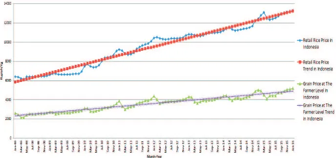
Trend Analysis of Retail Rice Price in Indonesia and Grain Prices at the Farmer Level in Indonesia The results of the retail rice prices trend analysis and the price of grain at the farmer level in January 2008 - January 2016 in Indonesia is shown in Figure 1.
Based on the results of trends analysis using the least squares method for retail rice prices trend in Indonesia during the period January 2008 - January 2016, it can be obtained the following equation.
Y1= 5,819.84 + 77.23X1...(9)
The intercept value (a1) obtained in the equation
showed that the estimated retail rice price in Indonesia in basis month of January 2008 reached Rp 5,819.84/kg. The trend coefficient trend (b1) showed that the estimated average retail rice price in Indonesia increased every month, amounting to Rp 77.23/kg. Based on the results, it could be identified that the retail rice price in Indonesia had an upward trend. This can be seen on the value of the trend coefficient (b1) which was positive.
Based on the trend analysis using the least squares method for grain prices at farmer level in Indonesia during January 2008 - January 2016 period,
the following equation could be obtained:
Y2= 2,342.42 + 26.62X2...(10)
The intercept value (a2) obtained in the equation
showed that the estimated price of grain at farmer level in Indonesia in basis month of January 2008 reached Rp 2,342.42/kg. The trend coefficient (b2)
showed the estimated average of increase in harvested dried grain prices at the farmer level in Indonesia every month, amounting to Rp 26.62/kg. Based on the results, it could be identified that the price of harvested dried grain at the farmer level in Indonesia had an upward trend. This could be seen from the trend positive coefficient value (b2).
The graph of retail rice prices in Indonesia and grain prices at farmer level in Indonesia had a similar pattern. Increasing the rice price at retail level (consumers) would be followed by an increase in producer prices (grain prices at farmer level). Grain price at farmer level was lower than the retail rice price in Indonesia. This was in line with Ariyani’s finding (2012) who found that the grain price (producers) was lower than rice price (consumers). This happens because there was a processing or changes in the form of grain to rice that would need production costs.
Vertical Integration Analysis of Rice Market in Indonesia
The results of the vertical integration analysis in Indonesian rice market were as follows:
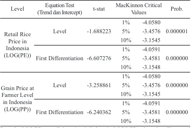
1) Stationary Test and the degree of integration The result of stationary test at the level (in level) for data retail rice prices Indonesia, as well as the price of grain (harvested dried grain) at farmer level, had an absolute value of t-statistic which was smaller than the absolute value of statistical MacKinnon at various levels of trust (1%, 5%, and 10%) on the
degree of integration of 0. This indicated that both data of retail rice prices and grain prices at farmer level in Indonesia produced time-series data that were not stationer or contained unit root or had a stochastic trend in the level or the degree of integration of 0. While the results of stationary test on the differentiation of the first data was the retail rice price in Indonesia and grain price at farmer level was stationer since the absolute value of the t-statistic was greater than the absolute value of statistical MacKinnon at various levels of trust (1%, 5%, and 10 %). This suggested that these two variables were
integrated in the first degree. The results of the stationary test were shown in Table 1.
2) Co-integration Test
Engle-Granger’s co-integration test was conducted to determine the existence of co-integration between variables of retail rice price with grain prices at farmer level in Indonesia. The results of Engle-Granger co-integration test were shown in Table 2.
Based on the estimated long-term equilibrium relationship of both variables, OLS could be obtained with the following equation:
LOG(PEt) = 0.512846 + 1.055191LOG(PPt)..(11)
Table 1.Summary of variables stationary test of retail rice prices and grain price (harvested dried grain) at farmer level in Indonesia
Remarks: LOG(PE) = retail rice prices in Indonesia, LOGO(PP) = log price of harvested dried grain at farmer level in Indonesia
Level Equation Test
(Trend dan Intercept) t-stat
MacKinnon Critical
Values Prob.
Retail Rice Price in Indonesia (LOG(PE))
Level -1.688223
1% -4.0580
0.000001
5% -3.4576
10% -3.1545
First Differentiation -6.607276
1% -4.0591
0.000000
5% -3.4581
10% -3.1548
Grain Price at Farmer Level in Indonesia
(LOG(PP))
Level -3.258861
1% -4.0580
0.000000
5% -3.4576
10% -3.1545
First Differentiation -6.240362
1% -4.0591
0.000000
5% -3.4581
10% -3.1548
Variable Symbol Coef. Prob.
C 0.512846 0.0090
LOG(PP) + 1.055191 0.0000
Adjusted R-squared = 0.954422 Prob (F-statistic) = 0.000000
Table 2.Estimated long-term equilibrium relationship of retail rice prices and price of grain (harvested dried grain) at farmer level in Indonesia.
Table 3.Residual testing for long-term equilibrium relationship of rice prices in Indonesia and the retail price of grain (harvested dried grain) at farmer level in Indonesia.
Variable Symbol Coef. Prob.
C 0.000314 0.9385
RESID01(-1) - 0.361139 0.0000
Adjusted R-squared = 0.173307 Prob (F-statistic) = 0.000015
Table 4.Estimation of short-term equilibrium relationship between retail rice prices and grain prices (harvested dried grain) at farmer level in Indonesia
Variable Symbol Coef. Prob.
C 0.005869 0.0000
D(LOG(PP)) + 0.259676 0.0000*
RESID01(-1) - 0.178021 0.0000*
Having obtained its long-term equilibrium relationship, the following step was to test the unit root on the residuals of Equation 11. Testing results of residual long-term equilibrium relationship between retail rice prices in Indonesia and grain price (harvested dried grain) at farmer level in Indonesia were shown in Table 3.
RESID01(-1) was the first differentiation of RESID01. The result from unit root test of the residuals was compared with the value of Critical Dickey-Fuller. If the absolute value of the t-statistic was smaller than the absolute value Critical Dickey-Fuller, H0 was accepted, which meant that there was co-integration. The value of t-statistic of RESID01(-1) was -4.573369. The absolute value of t-statistic > critical absolute value of Dickey-Fuller, so H0 was
rejected, which meant that there was co-integration. Moreover, the probability value of 0.0000 RESID01(-1) was less than the critical value of α = 0.05. This indicated that H0 was rejected, which meant that there was co-integration.
3) Co-integration Test and ECM
Having in mind that there was a co-integration between the retail rice price in Indonesia and grain price (harvested dried grain) at farmer level in Indonesia, ECM could be estimated. ECM analysis was conducted to determine the relationship between short-term balance of retail rice price and grain prices at farmer level in Indonesia. ECM test results were shown in Table 4.
Based on Table 4, the result of ECM regression was written as follows.
Δ(LOG(PEt)) = 0.005869 + 0.259676Δ(LOG(PPt))
– 0.178021(RESID01(-1)t) ...(12)
Statistically, the value of ECM was significant. This indicated that PE adjust the DPP with one lag. From Equation 12, it was known that the short-term elasticity of variable retail rice price in Indonesia was 0.259676, while the long-term elasticity on variable of retail rice price in Indonesia was 1.055191 (shown in Equation 11).
In testing the vertical integration of rice market in Indonesia by using Engle-Granger analysis and ECM, it was known that retail rice market in Indonesia is vertically integrated with grain producers in Indonesian market. This showed that transmission occurred between retail rice market price and grain producer market in Indonesia. The rice price would be transmitted properly from consumers to producers or vice versa, if there were a symmetry information between retail rice market and rice grain producers market in Indonesia.
CONCLUSION
Based on the analysis results, the conclusions of this study were as follows: Trend of retail rice prices in Indonesia and grain price (harvested dried grain) at farmer level in Indonesia were both in an upward trend; The vertical integration of rice market in Indonesia had a long-term equilibrium relationship and short-term equilibrium relationship.
ACKNOWLEDGMENT
Thank you to Dr. Slamet Hartono who have taught how to analysis using ECM method.
REFERENCES
Anonim. 2014. Beras. Bulletin of consumption of food 1stquarterly of Center for Data and
In-formation System of Agriculture. 5(1). http://pusdatin.sejen.pertanian.go.id [accessed at 15thSeptember 2015].
Ajija, S. R., D. W. Sari, R. H. Setianto and M.R. Pri-manti. 2011. Cara Cerdas Menguasai EViews. Jakarta: Salemba Empat Publisher.
Ariyani, D. 2012. Integrasi vertikal pasar produsen gabah dengan pasar ritel beras di Indonesia.
Manajemen Teknologi J.11(2): 225-238.
Gujarati, D.N and D.C. Porter. 2013. Dasar-dasar
Ekonometrika. 5thEdition. 2ndBook.
Transla-tor Raden Carlos Mangunsong. Jakarta: Mc-Graw-Hill Education (Asia) and Salemba Empat.
Ismet, M. 2010. Pelajaran dari krisis pangan dunia 2008. In: Arsitektur Kebijakan Beras di Era Baru. Bogor: PT IPB Press Publisher. Hermawan, A., M.D. Sarjana, Pertiwi and I.
Am-barsari. 2008. Informasi asimetris dalam transmisi harga gabah dan harga beras. Re-search and Development of Central Java
Province Journal.6(1): 61-72.
Nugroho, A. D., Jamhari and H.M. Jangkung. 2014.
Dampak AFTA terhadap perdagangan beras Indonesia. In: Ekonomi Perberasan Indone-sia. Bogor: Perhimpunan Ekonomi Pertanian Indonesia (PERHEPI).
Saleh, S. 2004. Statistik Deskriptif. Revision Edition. Yogyakarta: UPP AMP YKPN.
Subejo. 2014. Beras dan problematika pangan
na-sional. In: Ekonomi Perberasan Indonesia.
Bogor: Perhimpunan Ekonomi Pertanian
In-donesia(PERHEPI).
Yustiningsih, F. 2012. Analisis integrasi pasar dan transmisi harga beras petani-konsumen di
In-donesia. Thesis. Economic Faculty.