URBAN FLOODS MODELLING AND TWO-DIMENSIONAL SHALLOW WATER MODEL WITH POROSITY
Rudi Herman*
Abstrak
Pola genangan memiliki dampak yang sangat besar pada wilayah perkotaan di daerah dataran sungai. Dalam memperhitungkan perubahan dan pengurangan debit akibat adanya bangunan dan konstruksi yang lain pada wilayah dataran sungai, penggunaan model aliran dangkal dengan celah merupakan suatu hal yang diutarakan. Untuk hal ini model sumber air yang khusus untuk mengekspresikan kehilangan energi dalam wilayah perkotaan diperlukan. Formula yang diusulkan adalah membandingkan data uji coba yang diperoleh dari saluran laboratorium pada skala yang disesuaikan dengan wilayah perkotaan. Pada tingkat akurasi yang sama, metode ini memperlihatkan penurunan yang signifikan dalam perhitungannya dibandingkan dengan menggunakan grid yang lebih kecil pada simulasi klasik.
Kata kunci: dataran sungai, model fisik, model dua-dimensi
Abstract
Floodplains with urban areas have significant effects on inundation patterns. A shallow water model is presented, with porosity to account for the reduction in storage and in the exchange sections due to the presence of buildings and other structures in the floodplains. A specific source term representing head losses singularities in the urban areas is needed. The proposed formulation is compared to experimental data obtained from channel experiments on a scale of an urbanized area. The method is seen to result in significant reduction of computational effort compared to classical simulations using refined grids, with a similar degree of accuracy.
Keywords: inundation, physical model, two-dimensional model
* Staf Pengajar Jurusan Teknik Sipil Fakultas Teknik Universitas Tadulako, Palu 1. Introduction
Urban areas are often vulnerable because of the conjunction of a high
concentration of inhabitant and
economic actors and a hazardous context (impervious areas, proximity of rivers etc). A prevention approach leads to the development of flood mapping, with various applications in the field of
urban engineering: knowledge of
exposure to risk, regulation of urban
planning, elaboration of crisis
management scenarios for example. Among the existing numerical models, two-dimensional shallow water models seem to be the best compromise between flow description, data needs
and computational time. However, considering large urban areas can lead
to a dramatic increase of both
computational cell number and time. The use of large-scale models in such situations constitutes an alternative, because the required detailed meshing
of the urban area (to represent
representing head losses due to
singularities in the urban areas
(crossroads in particular) is needed. This specific source term is derived from general Borda head loss formula and takes the form of a tensor.
Depth and surface velocity
measurements have been conducted over a physical model of an urban area. These experimental data are compared
to various numerical simulations,
including classical bi-dimensional
simulation and different large-scale bi-dimensional simulations. Section 2 is devoted to a short presentation of the
governing equations of large-scale
models. Section 3 consists of the description of the physical model.
Section 4 treats the comparison
between experimental measurements and numerical results. Section 5 gives
some concluding and prospective
remarks.
directions respectively, Sfx and Sfy are the
source terms arising from energy losses in the x- and y- directions, respectively [3].
where zb is the bottom elevation. The first
term on the right-hand side eq. (3) account for the longitudinal variations in the porosity. The energy losses term is assumed to result from (i) the bottom and wall shear stress, accounted for by Strickler’s law and (ii) the energy losses triggered by the flow regime variations and the multiple wave reflections due to obstacles or crossroads, accounted for by classical head loss formulation. It can be written as;
………...(4)
Where K is the Strickler coefficient assumed to be isotropic in the following,
sxy, sxy, syx and syy are coefficients
accounting for the local head losses due
to urban singularities. These four
coefficients involved in a tensor are necessary to represent head losses in a street network not aligned on the system coordinates, Eq. (4) reduces to;
……….(5)
In what follows, Eq. (1) is
approach on unstructured grids with a Godunov-type scheme [4, 5]. A one-dimensional Riemann problem is defined in the local coordinate system attached to each interface. The flux vector in the direction normal to the interface is
computed using the following
procedure. In a first step, the Riemann problem in the global coordinate system is transformed to the local coordinates system. In a second step, the local Riemann problem is solved using a modified HLLC Riemann solver. Then the flux is transformed back to the global coordinate system. These numerical treatments are not detailed in this paper, see reference [3] for more details.
3.Description of the Physical Model
The experimental set-up is located in the laboratory of the Civil Engineering and Geoscience Department of the University of Newcastle Upon Tyne,
United Kingdom. The channel is
horizontal, 36 m long and 3.6 m wide, with a partly trapezoidal cross section as indicated in Figure-1. A gate is located placed in the channel, with a staggered layout. The Strickler coefficient of the
channel is equal to 100 m1/3/s.
Figure-1. Experimental set-up : channel dimensions (m) and urban district layout.
4. Comparison Between Experimental Measurement and Numerical Results
Two types of numerical simulations were undertaken:
A classical 2D simulation, where
buildings are represented as
impervious boundaries, and is
uniformly equal to 1.
A porosity 2D simulation, where is
equal to 1 everywhere except in the urban area where is strictly less than 1. The building are not explicitly represented in this simulation.
Various values of head losses
coefficients sx and sy were tested for
representing the influence of the street network. The porosity of the urban area was calculated as the ratio of the total plane area of the buildings to the area of the square delimiting the 22 buildings. This leads to a value of 0.45.
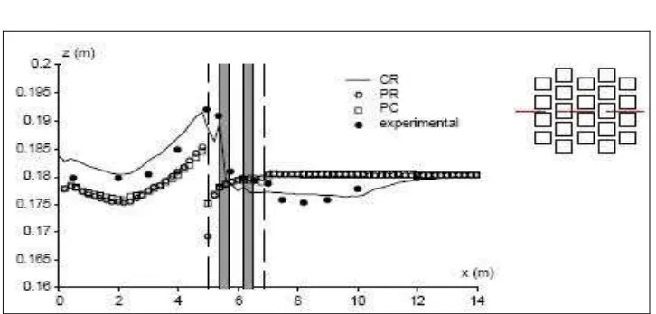
4.1 Influence of the meshing density of the urban area
Two porosity simulations have been compared, one with a refined meshing of the urban area, and the other with a coarse one. No local head losses are involved in this paragraph. In what follows, the different simulations will be recalled by two letters acronym, the first letter indicates the simulation type (Refined or Coarse). The channel was
divided into three zones, the
characteristic mesh lengths of which can be found in table-1. With the PR three simulations were plotted along the longitudinal axis y = 0, with the
experimental data (Figure-2). The
coefficient, or to use the local head-losses formulation of Eg. (4). The first solution is not physically appropriate because Strickler formulation is valid for
turbulent shear stress within the
boundary layer at the bottom and walls,
whereas local head-losses are assumed to be identical over the entire flow cross-section and should therefore simply be proportional to the square of the velocities involved [3].
Table 1. Characteristic mesh, cells number and computational time for each simulation.
Description CR PR PR
Upstream part
Downstream part except urban area Urban area
Total cells number
Computational time (400s simulated)
0.40 m 0.20 m 0.03 m 10335 132 mn
0.40 m 0.20 m 0.03 m 15299 200 mn
0.40 m 0.20 m 0.14 m 5549 63 mn
Figure 2. Simulated free surface profile without local head loss and depths along the axis y = 0
4.2 Influence of local head losses
Simulated free surface profiles (CR and PC) were compared with the experimental data but PC simulation
here involved local head-loss
coefficients. The various PC simulations
will be recalled by the code PC_sx-sy in
what follows. The coefficient sx of Eq. (5)
has been fixed greater than the
coefficient sy, because only the
transversal streets are continuous. The
computational time of all PC_sx-sy
simulations is approximately the same as given in the table-1. The following pairs
(sx-sy) have been tested: (10-5), (7-4),
(5-3) and (2-1). All the resulting simulated profiles are very close to the CR profile and experimental depths, but PC_5-3 appears to be the closest (Figure 3).
Compared to the various
paragraph results, it can be noted that the use of the local head-losses
coefficient leads to a clear
improvement of the simulated profile. The increase of the free surface profile before the city is well produced, but the drop after the city is under estimated. The three PC_10-5, PC_7-4, PC_5-3 simulations are very close to each other, so the sensitivity of the model to the two local head-losses coefficients is not very high.
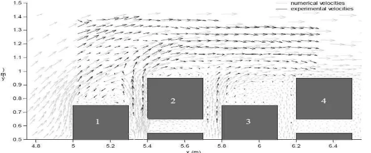
4.3 Comparison of the velocity fields The CR and PC_5-3 simulated velocity fields are compared to the one
obtained by the digital imaging
technique over the limited data
acquisitions window. It appears that experimental and CR velocity fields are very similar (Figure 4). The main flow skirting the city is well simulated, as well as the re-circulation zones located next to the buildings. The secondary flows existing the city through the transversal streets seem to be well represented too. Difficulties to have tracer particles in the right lower corner of the acquisition window are responsible of the lack experimental velocities in this zone. But it seems that the extension of the re-circulation zone between the building no. 2 and no.4 is under estimated in the CR simulation.
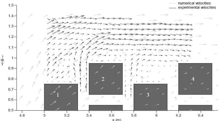
Experimental and PC_5-3 velocity fields are obviously very different inside the urban area, because of the absence of buildings in the PC simulation (Figure-5). But it is interesting to see that the use of porosity and local head-losses makes the flow mainly escaping from the entire channel. At a large scale, the
velocities can be considered as
correctly simulated with the PC_5-3 simulation.
Figure 5. PC_5-3 and experimental velocities fields.
5. Conclusions
A large-scale model has been used to simulate a steady flood flow through a simplified urban area. It has been
compared with both experimental
depth and velocity measurements, and classical two-dimensional model.
The large-scale model gives a good description of the main features of the flow (except inside the urban area), at a much lower computational cost than classical models. This illustrates the
possible operational uses of such
models, (i) large-scale simulation results may be used to provide boundary conditions to local models where the details of urban areas are represented, (ii) the simulation of floodplain featuring urbanized areas, but where the details of the flow within the urban areas are not of direct interest.
Further investigations are needed to express the components of the local head-losses tensor as functions of the geometrical characteristics of the urban area: buildings density, streets width, direction and slope.
6. References
Capart H., Young D.L., Zech Y.,2002, “
Voronoi imaging methods for the measurements of granular flows”. Experiments in Fluids, Vol. 32, No.1, 2002, pp 121-135.
Devina A., D’Alpaos L., Mattichio B.,2004,
“ A New Set of Equations for Very Shallow Water and Partially Dry Areas Suitable to 2D Numerical Domain”’ Proceedings Specially
Conference ‘Modelling of Flodd
Propagation Over Initially Dry
Areas’ Milano, Italy.
Guinot V., Soares-Frazao S., 2006, “Flux
and Source Term Discretization in Two Dimensional Shallow-Water Models With Porosity on Unstructured Grids”. Int.
Journal.’Numerical Methods in
Fluids, Vol 50, No.3, (2006), pp 309-345.
Guinot V., 2003, “Godunov-type
Hervouet J.,M., Samie R., Moreau B.,
2000, “Modelling Urban Areas in
DamBreak Flood Wave Numerical Simulations”, Proceeding of the
International Seminar and
Workshop on Rescue Based on Dambreak Flow Analysis, Seinajoki, Finland, (2000).
Toro E.F., 1997, “Riemann Solvers and