Volume 10 (2003), Number 1, 77–98
COMBINATORIAL HOMOLOGY IN A PERSPECTIVE OF IMAGE ANALYSIS
MARCO GRANDIS
Dedicated to Professor Hvedri Inassaridze, on the occasion of his seventieth birthday
Abstract. This is the sequel of a paper where we introduced an intrinsic ho-motopy theory and hoho-motopy groups for simplicial complexes. We study here the relations of this homotopy theory with the well-known homology theory of simplicial complexes. Also, our investigation is aimed at applications in image analysis. A metric spaceX, representing an image, has a structure of simplicial complex at each resolution ε >0, and the corresponding combi-natorial homology groupsHε
n(X) give information on the image. Combining
the methods developed here with programs for automatic computation of combinatorial homology might open the way to realistic applications. 2000 Mathematics Subject Classification:55N99, 68U10, 55U10, 54G99. Key words and phrases: Homology groups, image processing, simplicial complex, digital topology, mathematical morphology.
Introduction
This paper is devoted to the homology of simplicial complexes, its connections with the intrinsic homotopy theory developed in a previous work ([7], cited as Part I) and some methods of direct computation of combinatorial homology. As in Part I, the applications are aimed at image analysis in metric spaces, and connected with digital topology and mathematical morphology. In fact, a metric space X has a structure tεX of simplicial complex at each resolution
ε > 0, and the corresponding homotopy and homology groups πε
n(X), Hnε(X) detecting singularities which can be captured by an n-dimensional grid, with edges bound byε; this works equally well for continuous regions ofRnor discrete ones; in the latter case, our results are closely related with analyses of 0- or 1-connection in “digital topology” (cf. [11, 12, 2]). Such methods, combined with the use of recent computer programs for the homology of simplicial complexes, should be of use in the analysis of complicated 2- or 3-dimensional images, as produced by scanning a geographical region or an object; this work is under progress, and it would be difficult to say now whether it will produce results of practical interest: “realistic images” tend to produce big simplicial complexes, on which the existing programs for computing homology do not terminate in a reasonable time; but algorithms can be developed to reduce the size of the simplicial complex without changing its homology.
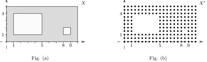
To give a first idea of these applications,in an elementary case, consider the subsetX ⊂R2 of Fig. (a), representing a planar image we want to analyse, for instance the map of a region
X
1 5 8 9
1 4 • • • • • • • • • • • • • • • • • • • • • • • • • • • • • • • • • • • • • • • • • • • • • • • • • • • • • • • • • • • • • • • • • • • • • • • • • • • • • • • • • • • • • • • • • • • • • • • • • • • • • • • • • • • • • • • • • • • • • • • • • • • • • • • • • • • • • • • • • • • • • • • • • • • • • • • • • • • • • • • • • • • • • • • • • • • • • • • • • • • • • • • • • • • • • • • • • • • X ′
1 5 8 9
1 4
Fig. (a) Fig. (b)
Viewing X as a topological space, we keep some relevant information which can be detected by the usual tools of algebraic topology; e. g. the fact thatXis path-connected, with two “holes”. However, we miss all metric information and are not able to distinguish a lake from a puddle. Further, if this “continuous” subspace X is replaced by a discrete trace X′ = X ∩ (ρZ×ρZ) scanned at
resolution ρ= 1/2, as in Fig. (b), we miss any topological information: X′ is a
discrete space.
It is more useful to view X and X′ as metric spaces (we shall generally use
thel∞-metric of the plane,d(x, y) = max(|x1−y1|,|x2−y2|), essentially because this is the metric of the categorical product R×R, cf. 1.2), and explore them at a variable resolution ε (0 6 ε 6 ∞). This will mean to associate to any metric space X a simplicial complex tεX at resolution ε, whose distinguished parts are the finite subsets ξ ⊂X with diam(ξ)6ε, and studythis complex by combinatorial homology.
Thus, the homology group Hε
1(X) = H1(tεX) of the metric space X, at resolution ε, allows us to distinguish, in Fig. (a): two basins at fine resolution (0 < ε < 1); then, one basin for 1 6 ε < 3; and finally no relevant basin at coarse resolution (ε > 3). The finite model X′ gives the same results, as
soon as ε > ρ; of course, if ε < ρ, i. e. if the resolution of the analysis is finer than the scanner’s, we have a totally disconnected object, in accord with a general principle: a “very fine” analysis resolution is too affected by the plotting procedure or by errors, and unreliable. Rather, the whole analysis is of interest, and can be expressed – as above – by some critical values (detecting metric characters of the image) together with the value of our invariant within the intervals they produce.
[image:2.595.150.498.152.257.2]to view it in this trivial form, as a collection of points. However, the categor-ical setting in [3] is much more general, and our methods might perhaps be presented in some form of that type.
Now, for a general overview of the present approach, let us recall that a simplicial complex, also called here a combinatorial space, is a set X equipped with a family of distinguished finite subsets, the linked parts, so that every subset of a linked part is linked and so are all singletons. Part I introduced intrinsic homotopies and homotopy groups for simplicial complexes, based on the standard (integral) line Z (1.3), the set of integers with linked parts con-tained in contiguous pairs {i, i+ 1}. A path in the simplicial complex X is precisely a map a : Z → X which is eventually constant on the left and the right. The set of paths P X inherits the simplicial structure from the hom-object XZ = Hom(Z, X) (the category of simplicial complexes being cartesian closed). Then, combinatorial homotopies are defined as maps α : X → P Y; this is more general than the classical contiguity relation (based on simplicial maps a : {0,1} → X), in an effective way: for instance, the integral line is contractible with respect to the present notion, while it is not so with respect to the equivalence relation spanned by contiguity (2.3).
Homology of simplicial complexes is a well known tool, intrinsically defined via oriented or ordered simplicial chains ([17], Ch. 4; [10], Ch. 2). Here, in Section 1, we prefer to use cubical chains, generated by the cubical set
T∗X = (TnX)n≥0 of links, the maps a : 2n → X defined over a power of the elementary integral interval 2 (the object on two linked points, 0 and 1). Section 2 deals with the interaction with combinatorial homotopies; the present homotopical invariance theorem for homology (2.4) is stronger than the clas-sical one, in as much as our homotopy relation is wider. For metric spaces, the derived metric combinatorial homology Hε
n(X) = Hn(tεX) satisfies, at a fixed resolution, the axioms of Eilenberg–Steenrod in an adapted form depend-ing on ε(2.6); it might be interesting to compare such groups with the Vietoris construction for compact metric spaces [18].
In Section 3, we consider various “comparisons”: thecombinatorial Hurewicz homomorphism, from homotopy to homology of simplicial complexes (3.1); the well-known canonical isomorphism from combinatorial homology to singular homology of the geometric realisation (3.2); and, in a particular case and up to degree 1, a canonical isomorphism from combinatorial homology to the singular homology of the open-spot dilation (3.4–5); the latter is a particular “dilation operator” considered in mathematical morphology (cf. [8]).
In Section 4, direct computations of combinatorial homology groups are given, using the Mayer–Vietoris sequence (1.6) and telescopic homotopies, a tool in-troduced in Part I to reduce combinatorial subspaces of tεRn to simpler ones (cf. 2.3). In particular, the examples of 4.3–4 should be sufficient to show how the study of the combinatorial homology groupsHε
n(X) of a metric subspace of
groups are far easier to compute. It is also relevant to note that the geometric realisation of these spaces is huge and of little help (cf. I.1.9). Finally, critical values for the family Hε
n(X) are briefly considered (4.4-5).
Notation. We use the same notation as in Part I. A homotopy α between the maps f, g : X → Y is written as α : f → g : X → Y. The usual bracket notation for intervals refers to the real or integral line, according to context. The letter κ denotes an element of 2 = {0,1} or S0 = {−1,1}, according to convenience; it is always written −, + in superscripts. The reference I.m, or I.m.n, or I.m.n.p, applies to Part I, and precisely to its sectionm, or subsection
m.n, or formula (p) in the latter.
1. On the Homology of Simplicial Complexes
After recalling the basic properties of simplicial complexes, we review their homology; this is constructed by means of cubical chains, based on the elemen-tary integral interval 2={0,1}.
1.1. Simplicial complexes. Asimplicial complex, also called here a combina-torial space (c-space for short), is a set X equipped with a set !X ⊂ PfX of
finite subsets ofX, calledlinked parts, which contains the empty subset, contains all singletons and is down closed: if ξ is linked, any ξ′ ⊂ξ is so. A morphism
of simplicial complexes, or map, or combinatorial mapping f : X → Y is a mapping between the underlying sets which preserves the linked sets: if ξ is linked in X, then f(ξ) is linked in Y. (Note that linked parts, here, are meant to express a notion of “proximity”, possibly derived from a metric; we shall generally avoid their usual name of simplices, as associated with a geometric realisation which is often inadequate for the present applications.)
As easily seen, the category Cs of combinatorial spaces is complete, co-complete and cartesian closed (I.1). The linked parts of a cartesian product
X1 ×X2 are the subsets of all products ξ1×ξ2 of linked parts; the exponen-tial Hom(A, Y) = YA, characterised by the exponential law Cs(X ×A, Y) =
Cs(X, YA), is given by the set of maps Cs(A, Y) equipped with the structure where a finite subset ϕ of maps A → Y is linked whenever, for all ξ linked in A, ϕ(ξ) =Sf∈ϕf(ξ) is linked in Y.
The forgetful functor | − | : Cs → Set has left adjoint D and right adjoint
C: the discrete structure DS is the finest (i. e., smallest) on the set S (only the empty subset and the singletons are linked), while thechaotic orcodiscrete structure CS is the coarsest (all finite parts are linked). Also D has a left adjoint, the functor
A subobject X′ ≺ X is a subset equipped with a combinatorial structure
making the inclusioni:X′ →X a map; equivalently, !X′ ⊂!X (this is the usual
notion of simplicial subcomplex [17]). The subobjects of X form a complete lattice: TXi (resp.
S
Xi) is the intersection (resp. union) of the underlying subsets, with structureT!Xi(resp.
S
!Xi). More particularly, a (combinatorial) subspace, orregular subobjectX′ ⊂X, is a subobject with the induced structure:
a part of X′ is linked iff it is so in X (the initial structure for i:X′ →X, i. e.
the coarsest one making i a map); any intersection or union of subspaces is a subspace. An equivalence relation R in X produces a quotient X/R, equipped with the finest structure making the projection X →X/R a map: a subset of the quotient is linked iff it is the image of some linked part ofX.
The category Cs∗
of pointed combinatorial spaces is also complete and co-complete.
1.2. Tolerance sets and metric spaces. Tol denotes the category of tol-erance sets, equipped with a reflexive and symmetric relation x!x′; the maps
preserve such relations. Equivalently, one can consider a simple reflexive unori-ented graph (as more used in combinatorics), or anadjacency relation, symmet-ric and anti-reflexive (as used in digital topology, cf. [11, 12]). The forgetful functor t : Cs → Tol takes the c-space X to the tolerance set over |X|, with
x!y iff {x, y} ∈!X; it has a left adjoint d and a right adjoint c : Tol → Cs. We are more interested in the latter: for a tolerance set A, cA is the coarsest combinatorial space over A inducing the relation ! (a finite subset is linked iff all its pairs are !-related); we shall always identify a tolerance set A with the combinatorial space cA. Thus,Tol becomes a full reflective subcategory of Cs, consisting of those c-spaces where a finite subset is linked iff all its parts of two elements are so. The embedding c preserves all limits and is closed under subobjects; in particular, a product of tolerance sets, in Cs, is a tolerance set.
A metric space X has a family of canonical combinatorial structures tεX, at resolutionε∈[0,∞], where a finite subsetξis linked iff its diameter is6ε. Each of them is a tolerance set, defined by x!x′ iff d(x, x′) 6 ε. The category Mtr
of metric spaces and weak contractions has thus a family of forgetful functors
tε :Mtr→Cs, trivial for ε = 0 (giving the discrete structure) andε=∞(the chaotic one). Marginally, and for ε >0, we also consider the “open” tolerance structure t−
εX defined by d(x, x′) < ε; but the family tεX yields finer results (cf. 3.4).
Unless otherwise stated, the real line R has the standard metric and the combinatorial structure t1R, with x!x′ iff |x− x′| 6 1. Beware of the fact that, in Mtr, a product has the l∞-metric, given by the least upper bound
d(x, y) = supidi(xi, yi); this precise metric has to be used if we want to “assess” a map into a product by its components: a mapping f : Z → QXi is a weak contraction if and only if all its componentsfi are so. Unless differently stated, the real n-space Rn will be endowed with the l
1.3. Combinatorial line and spheres. The set of integers Z, equipped with the combinatorial structure of contiguity, generated by all contiguous pairs
{i, i+ 1}, is called the standard (integral) line and plays a crucial role in our homotopy theory. It is a combinatorial subspace ofR and a tolerance set, with
i!j whenever i, j are equal or contiguous; all its powers and subobjects of pow-ers are tolerance sets. An integral interval has the induced structure, unless otherwise stated.
The structure of the standard (integral) n-space Zn ⊂ Rn is generated by the “elementary cubes” Qk{ik, ik+ 1}. As a crucial fact, the join and meet operations ∨,∧ :Z2 →Z are combinatorial mappings (while sum and product are not), as well as − : Z → Z; thus, Z is an involutive lattice in Cs. The standard elementary interval2= [0,1]∈Zis the chaotic c-space on two points, C{0,1}. The standard elementary cube 2n ⊂Zn is also chaotic, as well as the standard elementary simplexen = C{e
0, . . . , en} ⊂Zn+1, consisting of then+1 unit points of the axes (the canonical basis).
The discrete S0 = {−1,1} ⊂Z is the standard 0-sphere (pointed at 1, when viewed inCs∗
). There is no standard circle (I.6.6). But, for every integerk ≥3, there is a k-point circle, the quotient Ck = Z/ ≡k= {[0],[1], . . . ,[k−1]}, with respect to congruence modulo k; the structure is generated by the contiguous pairs{[i],[i+ 1]}; the base point is [0]; the homology groups are the ones of the circle (4.1; while the c-spaces similarly obtained for k = 1,2 are chaotic, hence contractible). Such circles are not homotopically equivalent, but related by the following maps, identifying two points
pk :Ck+1 →Ck, pk([i]) = [i] (i= 0, . . . , k), (1)
which are weak homotopy equivalences.
More generally, there is no standard n-sphere for n > 0. The simplicial (or tetrahedral) n-sphere ∆Sn ≺ Zn+2 has the same n+ 2 points of en+1 =
C(e0, . . . , en+1)⊂ Zn+2, but a subset is linked iff it is not total; the base point is e0. The cubical n-sphere Sn ≺ Zn+1 has the same 2n+1 points of the cube 2n+1 = C{0,1}n+1 ⊂ Zn+1, but the linked parts are the sets of vertices contained in some face of the cube, i.e. in some hyperplane ti = 0 or ti = 1; the base point is 0. The octahedral n-sphere ⋄Sn = {±e
0, . . . ,±en} ⊂ Zn+1 has 2n+ 2 points and the subspace structure: a subset is linked iff it does not contain opposed pairs ±ei; the base point ise0. Thus, ∆S0 ∼=S0 ∼=⋄S0 =S0, ∆S1 ∼=C3,S1 =∼⋄S1 ∼=C4. All these will be seen to behomological n-spheres (4.2).
Works in digital topology have considered various tolerance structures onZn; among the most used ones are the product structure, induced by thel∞-metric
(called 8-adjacency for Z2, because any point is linked to 8 others), and the structure t1(Zn, d1) induced by the l1-metric Σi|x
i−yi| (called 4-adjacency for
Z2); the fundamental group of regions of the latter has been considered in I.7.4.
inCs: faces(∂−, ∂+),degeneracy (e),connections (g−, g+) andsymmetries (the reversion r and the interchange s)
{∗} ∂
κ
2
e 2
2
gκ
r:2→2, s:22 →22, (1)
∂−
(∗) = 0, ∂+(∗) = 1, g−
(i, j) = max(i, j) =i∨j, g+(i, j) = min(i, j) = i∧j, r(i) = 1−i, s(i, j) = (j, i).
As a consequence, the endofunctor of 1-links orelementary pathsorimmediate paths in X
T(X) =X2 ={(x, x′
)|x!x′ ∈
X}, (x, x′
)!(y, y′
)⇔ {x, x′
, y, y′} ∈
!X, (2)
has natural transformations denoted by the same symbols and names
1
e T
∂κ gκ
T2 r:T →T, s:T2 →T2, (3)
which satisfy the axioms of a cubical comonad with symmetries ([5, 6]; or I.2.4). By cartesian closedness, the power Tn(X) = X2n
is the functor of n-links, or elementary n-paths a: 2n →X (n ≥0). Globally, such functors form a cubical object with symmetries T∗(X) (i= 1, . . . , n;κ∈2)
Tn(X) =X2n
, (4)
∂κ i =Tn
−i∂κTi−1 :Tn →Tn−1,
∂κ
i(a)(t1, . . . , tn−1) =a(t1, . . . , κ, . . . , tn−1),
ei =Tn−ieTi−1 :Tn−1 →Tn,
ei(a)(t1, . . . , tn) =a(t1, . . . ,ˆti, . . . , tn),
giκ =T n−i
gκTi−1 :Tn
→Tn+1, gκ
i(a)(t1, . . . , tn+1) =a(t1, . . . , gκ(ti, ti+1), . . . , tn+1),
ri =Tn−irTi−1 :Tn→Tn,
ri(a)(t1, . . . , tn) =a(t1, . . . ,1−ti, . . . , tn),
si =Tn−isTi−1 :Tn+1 →Tn+1,
si(a)(t1, . . . , tn+1) =a(t1, . . . , ti+1, ti, . . . , tn+1).
T∗(X) is a subobject of the cubical set with symmetries Sn|X|=|X|2
n
simi-larly obtained in Set, the cubical set of (elementary) cubes of the set |X|: the latter coincides with T∗(C|X|). Globally, we have a functor T∗ with values in
the category of cubical sets with symmetries.
1.5. Cubical combinatorial homology. Every cubical set A determines a collection Dn(A) = ∪iIm(ei : An−1 → An) of subsets of degenerate elements (with D0A =∅), yielding the normalised chain complex N :Cub→C∗Ab
where a∈An and ˆadenotes its class in the quotient.
The cubical chain complex of the simplicial complex X is the normalised chain complex C∗X = NT∗X, whose elements are the (normalised) cubical
chains of X
Σiλiaˆi ∈Cn(X) =F(TnX)/F(DnT∗X) (λi ∈Z, ai :2n →X); (2) we shall often write the normalised class ˆaas a, identifying all degenerate links to 0. We have thus thehomology of a combinatorial space
Hn :Cs→Ab, Hn(X) =Hn(C∗X) =Hn(NT∗(X)) (n >0). (3)
Relative homology is defined in the usual way. A combinatorial pair (X, A) consists of a subobjectA≺X (1.1): the subsetAhas a combinatorial structure finer than the restricted one so that the inclusion i : A → X is a map. We shall write Cs2 their category: a map f : (X, A)→ (Y, B) comes from a map f :X →Y whose restriction A→B is also a map.
The induced map on cubical sets i∗ : T∗A → T∗X is injective as well as
i∗ : C∗A → C∗X (a link in A is degenerate in X iff it is already so in A). We
obtain the relative chains of (X, A) by the usual short exact sequence of chain complexes
0 C∗A C∗X C∗(X, A) 0 (4)
therelative homology as the homology of the quotient,Hn(X, A) =Hn(C∗(X, A)),
and the natural exact sequence of the pair (X, A) from the exact homology se-quence of (4), with ∆n[c] = [∂nc]
· · · →HnA→HnX →Hn(X, A) ∆
→Hn−1A→ · · ·
→H0A →H0X →H0(X, A)→0. (5)
Plainly, C∗(X,∅) = C∗(X) and Hn(X,∅) = Hn(X). More generally, given a
combinatorial triple (X, A, B), consisting of subobjects B ≺A≺X, the snake lemma gives a short exact sequence of chain complexesC∗(A, B)C∗(X, B)։
C∗(X, A) and the exact sequence
· · · →Hn(A, B)→Hn(X, B)→Hn(X, A)→Hn−1(A, B)→ · · ·
→H0(X, A)→0. (6)
Plainly, the homology of a sum X = ΣXi is a direct sum HnX = ⊕HnXi (and every combinatorial space is the sum of its connected components, 1.1). It is also easy to see that ifX is connected (non empty), then H0(X)∼=Z (via the augmentation ∂e0 : C0X =F|X| → Z taking each point x ∈ X to 1 ∈ Z); thus, for every c-space X,H0(X) is the free abelian group generated by π0X.
1.6. Mayer–Vietoris and excision. Recall that, given two subobjectsU, V ≺
X, the structure of their union U ∪V is !U∪!V, while the structure of U ∩
V is !U∩!V (1.1). It follows easily that C∗ takes subobjects of X to chain
subcomplexes of C∗X, preserving joins and meets
C∗(U∪V) = C∗U +C∗V, C∗(U ∩V) =C∗U ∩C∗V. (1)
These facts have two important well-known consequences [17].
(a) The Mayer–Vietoris sequence. Let X =U ∪V be a combinatorial space (we shall say that X is covered by its subobjects U, V). Then we have an exact sequence
· · · −−−→ Hn(U∩V) (i∗,j∗)
−−−→ (HnU)⊕(HnV)
[u∗,−v∗]
−−−−→ Hn(X) ∆
−−−→ Hn−1(U ∩V) −−−→ · · · (2)
with the obvious meaning of round and square brackets; the maps u:U → X,
v :V →X, i :U ∩V →X, j : U ∩V → X are inclusions, and the connective ∆ is:
∆[c] = [∂na], c=a+b (a∈Nn(T∗U), b∈Nn(T∗V)). (3)
The sequence is natural, for a map f :X →X′
=U′∪
V′
, whose restrictions
U →U′, V →V′ are maps. (If our subobjects are subspaces, it is sufficient to
know that f U ⊂U′ and f V ⊂V′).
(b) Excision. Let a combinatorial space X be given, with subobjects B ≺
Y, A. The inclusion map i : (Y, B) → (X, A) is said to be excisive whenever !Y\!B =!X\!A (or equivalently: Y ∪A = X, Y ∩ A = B, in the lattice of subobjects of X). Then i induces isomorphisms in homology.
The proof is similar to the topological one, simplified by the fact that here no subdivision is needed. For (a), it is sufficient to apply the algebraic theorem of the exact homology sequence to the following sequence of chain complexes
0 −−−→ C∗(U ∩V)
(i∗,j∗)
−−−→ (C∗U)⊕(C∗V)
[u∗,−v∗]
−−−−→ C∗(X) −−−→ 0 (4)
whose exactness needs one non-trivial verification. Takea∈CnU,b∈CnV and assume that u∗(a) = v∗(b); therefore, each link really appearing in a (and b)
has image in U ∩V, and, by hypothesis, is a link there; globally, there is (one) normalised chain c∈Cn(U ∩V) such that i∗(c) = a, i∗(c) =b.
For (b), the proof reduces to a Noether isomorphism for the chain complexes
C(Y, B) = (C∗Y)/(C∗(Y ∩A)) = (C∗Y)/((C∗Y)∩(C∗A))
= (C∗Y +C∗A)/(C∗A) = (C∗(Y ∪A))/(C∗A) =C∗(X, A). (5)
2. Combinatorial Homotopy and Homology
2.1. Paths. A line of the combinatorial space X is a map a : Z → X, i.e. a sequence of points of X, written a(i) or ai, withai!ai+1 for all i∈Z. The lines of X form the combinatorial space L(X) =XZ; a finite set Λ of lines is linked iff each set ∪a∈Λ{ai, ai+1} is linked in X (fori∈Z).
A path (I.2.2) in X is a line a : Z → X eventually constant on the left and on the right: there is a finite interval ρ= [ρ−, ρ+]⊂Z (ρ− 6ρ+) such that a is constant on the half-lines ]− ∞, ρ−], [ρ+,∞[
a(i) =a(ρκ), for κi>κρκ (κ =±1), (1)
and determined by its values over ρ; the latter is called an (admissible) support of a. The end points of a, or faces ∂κa=a(ρκ), do not depend on its choice.
The path object P X ⊂XZ is the combinatorial subspace of paths. The path functor P :Cs→Csacts on a morphism f :X →Y as a subfunctor of (−)Z P f :P X →P Y, (P f)(a) =f a; (2)
the faces are natural transformations ∂κ : P → 1. The functor P is again a cubical comonad with symmetries (I.2.4), which is relevant for the study of homotopy. Here, we just need “first order properties” of homotopy, and it is sufficient to recall: thedegeneracy e: 1→P, taking a pointx to the constant path at x, e(x) : Z → X, and the reversion r : P → P, taking the path a to the reversed pathr(a) =−a:i7→a(−i).
Two pointsx, x′ ∈X are linked by a path inX iff x∼x′, for the equivalence
relation generated by the tolerance relation ! of X (1.1): π0X = |X|/ ∼ is indeed the set of path-components of X.
2.2. Homotopies. Classically (cf. [17, 3.5]), two maps f, g : X → Y are said to be contiguous if, for each ξ linked inX, f(ξ)∪g(ξ) is linked inY, i.e. if f!g
in the simplicial complex YX (1.1); a contiguity class of maps is an equivalence class generated by the previous relation. As in Part I, we shall use a wider notion of homotopy, the one deriving from the path functor P.
A homotopy of simplicial complexes (I.3.1) α : f → g : X → Y is a map
α : X → P Y such that ∂−α = f, ∂+α = g. It can also be viewed as a map
α : X → YZ, or α : Z×X → Y, such that every line α(x) admits a support ρ(x) = [ρ−(x), ρ+(x)] and
α(i, x) =f(x), for i6ρ−
(x), α(i, x) =g(x), for i>ρ+(x). (1)
On the other hand, general homotopies are represented by the path functor
P (as maps X → P Y), but cannot be corepresented (as maps IX → Y, for some object IX): the path functor has no left adjoint and there is no cylinder functor (in fact,P preserves finite limits, but does not preserve infinite products, I.2.4). The category Cs will always be equipped with general homotopies and the operations produced by the path functor, its degeneracy and reversion:
(a) whisker composition of maps and homotopies (for u: X′ → X, v : Y →
Y′):
v◦α◦u=vgu (v◦α◦u=P v.α.u:X′ →P Y′),
(b) trivial homotopies:
0f :f →f (0f =ef :X→ P Y),
(c) reversion:
−α:g →f (−α=rα:X →P Y).
Therefore, the homotopy relation f ≃ g, defined by the existence of a ho-motopy f →g, is a reflexive and symmetric relation, “weakly’ consistent with composition (f ≃g impliesvf u≃vgu), but presumably not transitive (related congruences are discussed in I.3.2). Two objects are homotopy equivalent if they are linked by a finite sequence of homotopy equivalences. The object X is contractible if it is homotopy equivalent to a point.
A deformation retract S of a combinatorial space X is a subspace whose inclusion u has a retraction p, withup≃idX
u:S ⇄X :p, pu= 1, α:up→1X, (2)
and we speak of a positive (resp. bounded, immediate) deformation retract when the homotopy α can be so chosen. Thus, an immediate deformation retractu:S ⊂X has a retractionp with (idX)!(up), i.e. ξ∪up(ξ) is linked for all ξ∈!X. An object is positively (resp. immediately) contractible if it admits a positive (resp. immediate) deformation retract reduced to a point; thus, X
is immediately contractible to its point x0 iff the latter can be added to any linked part (or is linked to any point, in a tolerance set). A non-empty chaotic space is immediately contractible to each of its points.
First, ifE denotes eitherZ orR(with thet1-structure) one can consider the homotopy
α: 0→id :E →E,
α(i, x) = 0∨(i∧x), α(i,−x) =−α(i, x) (x>0), (1)
whose general pathα(−, x) has a positive support, namely [0, ρ+(x)], with|x|6
ρ+(x)<|x|+ 1.
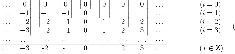
We call α a telescopic homotopy because it can be pictured as a collection of “telescopic arms” which stretch down, in the diagram below (forE =Z), at increasing i>0; the arm at x stabilities at depth ρ+(x) =|x|
. . . . . . . . . . . . . . . 0 −1 −2 −3 . . . 0 −1 −2 −2 . . . −01
−1 −1 . . . 0 0 0 0 . . . 01 1 1 . . . 0 1 2 2 . . . 0 1 2 3 . . . . . . . . . . . . . . . . . .
(i= 0) (i= 1) (i= 2) (i= 3)
. . . −3 -2 -1 0 1 2 3 . . . (x∈Z)
(2)
Note that there is no positive homotopy in the opposite direction id → 0. In fact, in the integral case, any positite homotopy β : id → f : Z → Z is necessarily trivial, since the map g =β(1,−) adjacent to id
. . . −2 −1 0 1 2 . . . (i= 0)
. . . g(−2) g(−1) g(0) g(1) g(2) . . . (i= 1) (3)
must coincide with the former (g(j) is linked withj−1, j, j+1, whenceg(j) =j), and so on. It is easy to see that the same holds in the real case. It follows that the only bounded deformation retract of the integral or real line is the line itself. Now, for then-dimensional spaceEn, atelescopic homotopy will be any prod-uct of 1-dimensional telescopic homotopies (centred at any point) and trivial homotopies. For instance, for n= 2, consider β =α×α(centred at the origin) and γ = 0id×α (centred at the horizontal axis)
β : 0→id:E2 →E2, β(i, x1, x2) = (α(i, x1), α(i, x2)), (4)
γ :p1 →id:E2 →E2, γ(i, x1, x2) = (x1, α(i, x2)), (5)
which show, respectively, that the origin and the horizontal axis are homotopy retracts ofE2.
Less trivially, to prove that the simplicial complex tεX ⊂ tεR2 described in Fig. (a) of the Introduction is contractible forε>3, we need ageneralised tele-scopic homotopy centred at the horizontal axis, with “variable vertical jumps” 1, 3, 1 (all6εand adjusted to jump over the two holes); for a precise definition, see I.3.6.
[image:12.595.139.518.251.338.2]Proof. Let us begin from animmediate homotopyα :f− →f+, represented by a mapα:2×X →Y. As forcubical singular homology [14], yields a homotopy of cubical sets
β :T∗f− →T∗f+:T∗X→T∗Y,
βn :TnX →Tn+1Y, βn(a:2n→X) =α◦(2×a) :2n+1 →Y;
(1)
in fact, fora∈TnX, b∈Tn−1X, 16i6n, andκ= 0,1 (−,+ in superscripts) (∂κi+1βna)(t1, . . . , tn) =α◦(t1, a(t2, . . . , κ, . . . , tn)) = (βn−1∂κia)(t1, . . . , tn),
(∂1κβna)(t1, . . . , tn) =α◦(κ, a(t1, . . . , tn)) = (fκa)(t1, . . . , tn), (βneib)(t1, . . . , tn+1) =α◦(t1, b(t2, . . . ,ˆti+1, . . . , tn+1)) =
= (ei+1βn−1b)(t1, . . . , tn+1).
(2)
Then β produces a homotopy of the associated normalised chain complexes
γn :CnX →Cn+1Y, γn(Σiλiaˆi) = Σiλi(βn(ai))ˆ. (3) Now, a bounded homotopy is a finite concatenation of immediate ones, and produces again a homotopy of chain complexes. Finally, for a general homotopy, it suffices to recall that combinatorial homology has finite supports (1.5), and that each homotopy on a finite domain is bounded (2.2).
2.5. Reduced homology and the elementary suspension. Simplicial com-plexes have an elementary suspension ΣX, which plays the role of a homo-logical suspension, i.e. a functor Σ : Cs → Cs with a natural isomorphism
hn : Hen(X) = Hen+1(ΣX), in reduced homology. (Its topological analogue is McCord’s non-Hausdorff suspension, [15, Section 8].)
The augmented cubical chain complex Ce∗X has a component C−1(X) =Z, with augmentation ∂e0 : C0X =F|X| → Z taking each point x ∈ X to 1∈ Z. Its homology is the reduced homology of X
e
Hn:Cs→Ab, Hen(X) =Hn(Ce∗X) (n>−1). (1)
Let Z∗ = Ce∗(∅) be the chain complex reduced to one component Z, in
de-gree −1. The obvious short exact sequence Z∗ Ce∗X ։ C∗X produces an
exact homology sequence, which reduces to a four-term exact sequence in low dimension and a sequence of identities for n>1
0→He0(X)→H0(X)→Z→He−1(X)→0, Hen(X) =Hn(X). (2)
Thus, also He0(X) is free abelian. If X is empty, all homology and reduced homology groups vanish, except forHe−1(∅) =Z. In the contrary,∂e0 :F|X| →Z is surjective andHe−1(X) = 0: the sequence in (2) splits asH0(X)∼=He0(X)⊕Z.
Reduced homology also has a Mayer–Vietoris sequence, which ends in degree
−1, proved in the same way; but note that it does not preserve sums.
ΣX is covered by two subspaces, the lower and upper elementary cones
C−
X =X∪ {−∞}, u+ :X ⊂C−
X, ∂−
:{∗} →C−
X, ∗ 7→ −∞, C+X =X∪ {+∞}, u−
:X ⊂C+X, ∂+ :{∗} →C+X, ∗ 7→+∞,
(3) which are immediately contractible to their vertex κ∞ (2.2). Since their
inter-section is X, the Mayer–Vietoris sequence of ΣX in reduced homology gives a natural isomorphism (for n>−1)
∆n+1 :Hen+1(ΣX) =Hen(X), ∆n+1[c] = [∂n+1a], (4)
where c=a+b, a∈Cn+1(C−X) andb ∈Cn+1(C+X).
The isomorphism sn = (−1)n+1(∆n+1)−1 : Hen(X) = Hen+1(ΣX) has a more canonical description: it is induced by the following chain map ¯s∗ of degree 1
¯
s−1 :Ce−1X =Z→C0(ΣX), 17→(−∞)−(+∞), ¯
sn :CnX →Cn+1(ΣX), (a:2n→X)7→a−−a+ (n >0),
aκ :2n×2→CκX ⊂ΣX, aκ(t,0) =a(t), aκ(t,1) =κ∞
, ∂(a−
−a+) = (Σi,κ(−1)i+κ∂iκ(a
−
−a+)) + (−1)n+1(a−a) = (∂a)−
−(∂a)+ (i6n; κ=±).
(5)
Since we already know that ∆n+1is iso, it is sufficient to check that ∆n+1·sn= (−1)n+1id on each homology class [Σλ
iai] (∂(Σλiai) = 0)
∆n+1·sn[Σλiai] = ∆n+1[Σλi(a−i −a +
i )] = [Σλi∂(a−i )]
= [(Σλi∂ai)−] + (−1)n+1[Σλiai] = (−1)n+1[Σλiai]. (6)
We end with some formal remarks. The elementary lower cone C−X comes
with an immediate homotopy δ− : ∂−p → u+ : X → C−X from the vertex
to the basis, which is universal for all immediate homotopies f → g : X → Y
where f is constant (factors through the point); symmetrically for C+X. The elementary suspension comes with a homotopyof support [−1,1])
σ:∂−
→∂+ :X →ΣX, σ(−1, x) =−∞,
σ(0, x) = x, σ(1, x) = +∞, (8)
which is universal for all homotopies of support [−1,1], between constant maps defined on X.
But there is no standard cone and no standard suspension, representing ho-motopies of the previous kinds without restrictions on supports. In fact, and loosely speaking, the cone or the suspension of the singleton would produce a standard interval Iand a cylinder functor I×(−), which we already know not to exist. (For a precise proof, one can adapt the argument of I.6.5 showing that the pointed S0 has no suspension in Cs∗
2.6. Metric combinatorial homology. Metric spaces inherit a family of ho-mology theories (metric combinatorial homology at resolutionε) via the functors
tε :Mtr2 →Cs2 Hε
n :Mtr2 →Ab, Hnε(X, A) =Hn(tεX, tεA) (0< ε <∞), (1) on the obvious category Mtr2 of pairs (X, A) of metric spaces (A ⊂ X with the induced metric).
The axioms of Eilenberg–Steenrod are satisfiedin an adapted form depending on ε (for excision):
- the functoriality and dimension axioms hold trivially;
- exactnessandnaturalityfor the homology sequence of a pair (X, A) come from the similar properties (1.5) for the combinatorial pair (tεX, tεA); - homotopy invariance holds for homotopies α : ([0,1]×X,[0,1]×A)→
(Y, B) inMtr2; in fact, choose a finite partition 0 = t0 <· · ·< tk= 1 of the standard interval such that ti−ti−1 6ε; then α produces a combi-natorial homotopy (actually inTol2), with bounded support [0, k]⊂Z
β : (Z×tεX,Z×tεA)→(tεY, tεB), β(i, x) =α(t(i∨0)∧k, x), (2) since |i−i′|61 andd(x, x′)6ε implies d(β(i, x), β(i′, x′))6ε;
- finally, theexcision isomorphismHε
n(X\U, A\U)→Hnε(X, A) holds for metric subspaces U ⊂A ⊂X, provided that: if x ∈U and d(x, x′)6 ε,
then x′ ∈ A; in fact, under this condition, the combinatorial inclusion
map (tε(X \U), tε(A\U)) = (tεX, tεA) is excisive (1.6b): if ξ is linked inX either it is contained inX\U, or there is somex∈ξ∩U; but then
ξ⊂A.
3. Comparison Homomorphisms
We deal now with the combinatorial Hurewicz homomorphism from homotopy to homology (3.1) and the canonical isomorphism from combinatorial homology to the singular homology of a realisation, either the well-known geometric one (3.2), or the “open-spot dilation” (in a particular case, 3.4-5).
3.1. The combinatorial Hurewicz comparison. Let X be a pointed com-binatorial space. There is a natural Hurewicz homomorphism, for n> 1
hn :πn(X)→Hn(X), [a]7→[Σiai],
ai :2n →X, ai(j) = a(i+j) (i∈Zn),
(1)
where a : Zn → X is a net with trivial faces, all a
i : 2n → X are links (degenerate except for finitely many indices i, belonging to the support of a), and the normalised chain Σiai is a cycle.
Similarly, for a combinatorial space X,
h0 :π0(X)→H0(X), [a]7→[a], (2)
is a mapping of sets, and actually the canonical basis of the free abelian group
It should not be difficult to prove directly the Hurewicz theorem for combina-torial homotopy and homology, adapting the classical proof of the topological case; but we shall deduce it from the latter (in 3.3), via the geometric compar-isons in homotopy (I.6.6) and homology (below).
3.2. The geometric comparison in homology. Let X be a combinatorial space, RX its geometric realisation. As proved in [17], there is a natural
iso-morphism (geometric comparison)
Φn :Hn(X)→Hn(RX), Φn[Σikiai] = [Σikiˆai], (1)
from combinatorial homology to (singular) homology, which we adapt now to cubical chains.
The geometric realisation RX is the set of all mappings λ : X → [0,1]
with linked support supp(λ), such that Σxλ(x) = 1. X is embedded in RX,
identifyingx∈Xwith its characteristic function. A point ofRX can be viewed
as a convex combination λ= Σiλixi of a linked family of X; each (non-empty) linked subset ξ havingp+ 1 points spans a simplex
∆(ξ) ={λ∈RX | supp(λ)⊂ξ}. (2)
All ∆(ξ) are equipped with the euclidean topology (via a bijective correspon-dence with the standard simplex ∆p, determined by any linear order ofξ), and
RX with the direct limit topology defined by such subsets: a subset of RX is
open (or closed) if and only if it is so in every ∆(ξ). (This is generally known in the literature as the weak or coherent topology, as distinct from the metric topology, cf. [17, p. 111]). Each ∆(ξ) is closed in RX. The open simplex
∆◦(ξ) = {λ∈RX | supp(λ) = ξ}is open in ∆(ξ);RX is the disjoint union of
its open simplices.
The image of a link a : 2n → X is a linked subset ξ of X, contained in the convex space ∆(ξ) ⊂ RX, and we can consider the multiaffine extension
ˆ
a: [0,1]n →RX of a (separately affine in each variable). This transformation, plainly consistent with faces and degeneracies, defines a natural homomorphism (1), which is proved in [17] to be iso.
If X is pointed or n = 0, this comparison is coherent with the similar iso-morphism Φn :πn(X)→πn(RX) constructed in I.6.6: we have a commutative
diagram
πn(X) Φn
−−−→ πn(RX)
hn
y
yhn
Hn(X) Φn
−−−→ Hn(RX)
(3)
with the Hurewicz mapshn, the combinatorial one at the left (3.1) and the usual, topological one, at the right. This diagram is natural, for maps f :X →Y in
Cs∗
3.3. Corollary. (a) (Hurewicz)LetX be a pointed combinatorial space. IfX is
n-connected (πk(X) trivial for 06k 6n), then Hk(X) = 0 for 0< k 6n and
hn+1 : πn+1(X) →Hn+1(X) is iso (or, for n = 0, induces an iso ab(π1(X))→
H1(X)from the abelianised group).
(b) (Whitehead) If f : X → Y is a map of connected pointed simplicial complexes and πk(f) is an isomorphism for 1 6 k 6 n, the same holds for
Hk(f).
(c) (Whitehead) If f : X → Y is a map of non empty simplicial complexes and for all x ∈ X, πk(f) : πk(X, x) → πk(Y, fx) is an iso for 0 6 k 6 n, the same holds for Hk(f).
Proof. (a) Apply the usual (topological) Hurewicz theorem to the commutative diagram 3.2.3.
(b) Again in the diagram 3.2.3 (natural on f), apply a theorem of J.H.C. Whitehead [9, p. 167] saying that, if a map g :S→T between path-connected pointed spaces induces an iso on the k-homotopy groups, for 1 6 k 6 n, the same holds for singular homology. (There is also a modified version, where one assumes thatπk(f) is an iso for 1 6k < nand epi fork =n, and concludes the same for Hk(f). Both facts are easily deduced from the exact homotopy and homology sequences of the pair (Mf, X) based on the mapping cylinder of f, linked by Hurewicz homomorphisms.)
(c) Follows from the previous point, via direct sum decomposition over
path-components.
3.4. The open-spot dilation. Let X be a metric space and ε >0. First, we want to compare the tolerance structures tεX and t−εX, where two points are linked iff their distance is 6 ε or < ε, respectively (1.2). As is the case for homotopy groups, the homology groups of the first family determine the ones of the second (but not vice versa, cf. I.7.3)
Hn(t−
εX) = colimη<εHn(tηX), (1)
as a trivial consequence of the finiteness of links: a mapa:2n→t−
εX is also a map 2n →t
ηX, for η= diam(a(2n))< ε.
Now, let X be a metric subspace of a normed vector space E and ε > 0. Recall (from I.7.4) that the open-spot realisation D−
ε(X) of X inE (a dilation operator considered in mathematical morphology, cf. [8]) is the subspace of E
formed by the union of all open d-discs centred at points of X, of radius ε/2 (pointed at the base-point of X, if X is pointed)
D−
ε (X) = D
−
ε(X, d) ={x
′
∈E |d(x, x′
)< ε/2 for some x∈X} ⊃X. (2) Say that X is t−
ε-closed (resp. tε-closed) in E if Dε−(X) contains the convex envelope of all linked subsets of t−
εX (resp. tεX), so that there is a continuous mapping
f−
ε :R(t
−
εX)→D
−
ε(X) (resp. fε:R(tεX)→D−ε(X)), (3) extending the identity ofXand affine on each simplex ∆(ξ) of the domain. Note that, ifXistε-closed, then it is alsot−
ε-closed andf
−
ε = (R(t
−
D−
ε(X)) factors as the map induced by the subobject-inclusion t−εX ≺ tεX followed by fε.
3.5. Theorem (Open-spot comparison isomorphisms in homology).
(a)IfX ist−
ε-closed in E, there is a canonical isomorphismΨ
−
n :Hn(t
−
εX)→
Hn(D−
ε X)between the combinatorial and topological homology groups, which is the composite of the geometric realisation isomorphism Φn (3.2) with an iso-morphism induced by the “affine” map f−
ε
Φ−
n =Hn(f
−
ε )·Φn= (Hn(t
−
εX)→Hn(R(t
−
εX))→Hn(D
−
εX)) (n 61). (1)
(b) If X is also tε-closed, there is a canonical isomorphism Ψn :Hn(tεX)→
Hn(D−
ε X)consisting of the lower row of the following commutative diagram of isomorphisms
Hn(t−
εX) Φn
−−−→ Hn(R(t−
εX))
Hn(fε−)
−−−−→ Hn(D−
ε X)
y
y
Hn(tεX) Φn
−−−→ Hn(R(tεX)) −−−−→Hn(fε) Hn(D−
ε X)
(1)
(the two vertical arrows being induced by the inclusion t−
εX ≺tεX).
Proof. Let X be t−
ε-closed (resp. tε-closed) in E. As proved in theorem I.7.5, the homotopy homomorphismπn(f−
ε , x) (resp. πn(fε, x)) is an isomorphism, for all x ∈X and n 6 1. From the Whitehead theorem (the classical, topological one, in form 3.3c) it follows that Hn(f−
ε ) (resp. Hn(fε)) is iso, forn 61. Combining this with the geometric comparison Φn (3.2), we have the thesis.
4. Computation of Combinatorial Homology
In this section some computations of homology are given, either directly via the intrinsic Mayer–Vietoris (M-V) sequence, or via the geometric realisation; in some cases, one might similarly use the open-spot dilation (3.4-5). The results in 4.3-4 are used as a support for image analysis.
4.1. Homological circles. All the circles Ck (k > 3; 1.3) are homological 1-spheres, since their geometric realisation is the circle. But the homology is also easily computed by the M-V sequence (1.6).
(a) If k > 3, Ck is covered by two subspaces U, V which are contractible (being isomorphic to integral intervals) and whose intersection is the discrete object on two points, e.g.
U ={[0],[1],[2]}, V ={[2], . . . ,[k−1],[0]}, (1)
so that, taking into account the homology of a sum and the invariance theo-rem (2.4), the computation on the M-V sequence proceeds precisely as for the topological circle.
Then,U and V are contractible andU∩V acquires the discrete structure. One concludes as above.
The naturality of the M-V sequence proves also that all mapspk:Ck+1 →Ck induce isomorphism in homology (by the Five Lemma); this suggests that it might be useful to realise a “standard circle” as a pro-object (cf. I.6.5).
4.2. Homological spheres. The n-sphere ∆Sn ≺ en+1 (1.3) has the same homology as the topological n-sphere, since its geometric realisation is homeo-morphic to the standard (topological) sphereSn. Our result can also be proved by induction, as in the topological case, covering ∆Sn(n >1) with the following subobjects (a face of the standard simplex and the union of all the others)
U =en=C{e
0, . . . , en} ⊂∆Sn, V ≺∆Sn ≺en+1, (1)
where V has the same underlying set {e0, . . . , en+1} as ∆Sn, and all its linked sets except U. Then, U ∩V = ∆Sn−1.
For the cubicaln-sphereSn ≺2n+1 (whose geometric realisation is a space of dimension 2n−1, having the homotopy type of then-sphere), the direct proof is similar: cover Sn (n > 1) with the following subobjects (again, a face of the standard cube and the union of all the others)
U =2n =C{0,1}n⊂
Sn, V ≺Sn≺2n+1, (2)
where V has the same underlying set {0,1}n as Sn, and all its linked sets except U. Again,U ∩V =Sn−1.
Finally, the octahedral n-sphere⋄Sn={±e
0, . . . ,±en} ⊂Zn+1 has again for geometric realisation then-sphere. But it suffices to recall that⋄Sn= ΣnS0 and apply the suspension isomorphisms (2.5); or also, to apply M-V to the following subspaces U, V, which are immediately contractible to ±en
U =⋄Sn−1∪ {−e
n}, V =⋄Sn−1∪ {en}, U ∩V =⋄Sn−1. (3)
4.3. Metric combinatorial homology and image analysis. The homology at variable resolution Hε
n(X) = Hn(tεX) of a metric subspace X ⊂ (Rn, d∞)
can often be computed directly (as its fundamental group in Part I), using the telescopic retracts introduced in I.3 and the M-V sequence (instead of the van Kampen theorem). This can be of interest within image analysis, as showed by the examples below. Of course, Hε
Let us consider, as in I.7.1.2, the closed region X = T \(A∪B∪C) of the real plane (with the l∞-metric), endowed with thetε-structure (>0)
X
1 4 8 10
1 2 5
A
B C
T = [0,11]×[0,5]
A=]1,4[×]1,4[
B = [4,8]×]1,2[
C=]8,10[×]1,3[
(1)
Then, the same coverings and telescopic homotopies used in I.7.1 for πε 1(X) show that Hε
0(X) ∼= Z and Hnε(X) = 0 for all n > 1, while the first homology group gives:
H1ε(X)∼=Z (0< ε <1; 26ε <3), Z2 (16ε <2), 0 (36ε6∞), (2) the generators being provided by the 1-chains associated to the loops which generate πε
1(X) (I.7.1). These results (including the description of generators) give the same analysis of the metric space X as provided by the fundamental group (I.1.8): at fine resolution (0 < ε < 1), our map presents one basin
A∪B∪C; thentwo basinsA, Cconnected by a bridgeable channelB (16ε <2); or one basin A with a negligible appendix (26 ε < 3); and finally no relevant basin (ε > 3). Also here, the finite model X ∩(ρZ×ρZ), resulting from a scanner at resolution ρ = k−1 (for an integer k > 2, in order to simplify the interference with the boundary ofX), has the same homology groups for ε>ρ
(and the same analysis).
Similarly, one proves that the solid metric subspaceX′ =T′\(A′∪B′∪C′)⊂ R3, where
T′ = [0,11]×[0,5]2, A′ =]1,4[×]1,4[2,
B′ = [4,8]×]1,2[2, C′ =]8,10[×]1,3[2, (3) equipped with the tε-structure (ε > 0), has Hε
0(X) ∼= Z, Hnε(X
′
) = 0 for all other n6= 2, and
Hε 2(X
′
)∼=Z (0< ε <1; 26ε <3), Z2 (16ε <2), 0 (36ε6∞). (4) The analysis is analogous to the previous one, 1 dimension up: our object presentsone cavity A′∪B′∪C′, at resolution 0< ε <1; thentwo cavitiesA′, C′
connected by a thin channel (1 6 ε < 2); or one cavity A′ with a negligible
appendix (26ε <3); and finally no relevant cavity (ε>3).
4.4. Critical values. Considering the previous examples, one is lead to con-sider the variation of the system of homology groups Hε
n(X) → Hnη(X) (0 6
ε 6 η 6 ∞), for a metric space X, through its critical values (cf. Deheuvels [4], Milnor [16]).
[0,∞]. In the contrary, ε is a left critical (resp. right critical, critical) value; and a bilateral critical value if it is both left and right critical.
Thus, in dimension 1, the metric space X considered in 4.3.1 has a right critical value at 0 and left critical values at 1, 2, 3. The metric subspace
Y =T \(A∪B) ⊂R2 represented below has a right critical value at 0 and a bilateral critical value at 2
1 3 8 10
1 4
A B
T =[0,11]×[0,4]
A=]1,3[×]1,3[
B =[8,10]×[1,3]
(1)
Hε
1(Y)∼=Z2 (0< ε <2), Z (ε= 2), 0 (ε >2), (2) since its homology groups can be computed by the same techniques as above (cf. I.7.2).
4.5. Proposition. For a general metric spaceX, assume that the real interval
K = [ε, η] ⊂ [0,∞] does not contain any critical value in dimensions n −
1, n, n+ 1 (except possibly a left critical value at ε and a right one at η). Then
Hε
n(X)→Hnη(X) is an isomorphism (but not vice versa, cf. 4.3.2).
Proof. K is compact and every p ∈ K has a K-neighbourhood where the ho-mology system is constant, in the given degrees; by the Lebesgue covering theorem, one can find a finite partition of K, ε = p0 < p1 < · · · < pk =
η, whose intervals [pi−1, pi] are contained in such neighbourhoods. Thus all
Hm(tpi−1X)→Hm(tpiX) are iso (m =n−1, n, n+ 1), and the relative
homolo-giesHm(tpiX, tpi−1X) are null, form=n, n+1, by the exact homology sequence
of a pair. The exact homology sequence of the triple (tpi+1X, tpiX, tpi−1X) shows
then that also Hm(tpi+1X, tpi−1X) = 0, in the same degrees m =n, n+ 1 (0 < i < k). Similarly, by finite induction,Hm(tηX, tεX) = 0 form=n, n+1; finally, the thesis follows from the exact homology sequence of the pair (tηX, tεX).
Acknowledgements
This work is supported by MIUR Research Projects.
References
1. K. Borsuk,Concerning homotopy properties of compacta.Fund. Math. 62(1968), 223–254.
2. L. Boxer, A classical construction for the digital fundamental group. J. Math. Imaging Vision10(1999), 51–62.
3. J. M. CordierandT. Porter,Shape theory: categorical methods of approxima-tion.Ellis Horwood, Chichester, 1989.
4. R. Deheuvels, Topologie d’une fonctionelle.Ann. of Math. (2) 61(1955), 13–72. 5. M. Grandis, Cubical monads and their symmetries.Proc. of the Eleventh Intern.
6. M. Grandis, Cubical homotopical algebra and cochain algebras. Ann. Mat. Pura Appl.170(1996), 147–186.
7. M. Grandis,An intrinsic homotopy theory for simplicial complexes, with applica-tions to image analysis.Appl. Categ. Structures10(2002), 99–155.
8. H. J. A. M. Heijmans, Mathematical morphology: a modern approach in image processing based on algebra and geometry.SIAM Rev.37(1995), 1–36.
9. S. T. Hu,Homotopy theory.Academic Press, New York,1959.
10. P. J. HiltonandS. Wylie,Homology theory.Cambridge Univ. Press, Cambridge, 1962.
11. T. Y. Kong, R. Kopperman,andP. R. Meyer,A topological approach to digital topology.Amer. Math. Monthly98(1991), 901–917.
12. T. Y. Kong, R. Kopperman, and P. R. Meyer Eds., Special issue on digital topology.Topology Appl. 46(1992), No. 3, 173–303.
13. S. Mardeˇsi´c and J. Segal, Shape theory: the inverse system approach. North-Holland Mathematical Library, 26.North-Holland Publishing Co., Amsterdam-New York,1982.
14. W. Massey, Singular homology theory. Graduate Texts in Mathematics, 70. Springer-Verlag, New York-Berlin,1980.
15. M. C. McCord,Singular homology groups and homotopy groups of finite topolog-ical spaces.Duke Math. J. 33(1966), 465–474.
16. J. W. Milnor, Morse theory. Annals of Mathematics Studies, No. 51. Princeton Univ. Press, Princeton, N.J.,1963 .
17. E. H. Spanier, Algebraic topology. McGraw-Hill Book Co., New York-Toronto, Ont.-London,1966
18. L. Vietoris,Uber den h¨¨ oheren Zusammenhang kompakter R¨aume und eine Klasse von zusammenhangstreue Abbildungen.Math. Ann.97(1927), 454–472.
(Received 28.05.2002; revised 14.12.2002)
Author’s address:
Dipartimento di Matematica Universit`a di Genova
Via Dodecaneso, 35, 16146-Genova Italy