M – 33
A STUDY OF ARIMA AND GARCH MODELS
TO FORECAST CRUDE PALM OIL (CPO) EXPORT IN INDONESIA
Sapto Rakhmawan*, Khairil Anwar Notodiputro, I Made Sumertajaya
Statistics Department, FMIPA, Bogor Agricultural University, Indonesia *Correspondence to: [email protected]
Abstract
Indonesia is the biggest exporter Crude Palm Oil (CPO) country in the world. In 2013, export of Indonesian CPO reach $ 15.84 billion. CPO is important for various things, such as cooking oil, vegetable fat for milk and ice cream, raw materials of soap or cosmetics industry, or alternative fuels. The export of CPO is very important for the national economic development since it contributed significantly to the trade balance of Indonesia. Therefore, in order to support the government in making the right policy, forecasting export of CPO is necessary.
In this study, a series of CPO export data was analyzed using time series analysis and forecasting techniques. Two classes of models were investigated, namely ARIMA models and GARCH models, and the comparison of the models was reviewed. The data used in this study were monthly export registration data, available at various ports for export across Indonesia from 1996 to 2013.
The results showed that the first model was suitable for time series data with constant variance and hence if the problem of variance heterogeneity existed in the data, then a transformation to the data was required. The second model, on the other hand, was suitable for time series data having serious problems with heterogeneity of variance. However, in this study it was shown that a simple transformation of ARIMA models has fitted the data properly and could overcome the heterogeneity of variance problems.
Key words: CPO, ARIMA, log transformation, GARCH, forecasting
INTRODUCTION
Indonesia is the biggest country in the world in exporting Crude Palm Oil (CPO). In 2013, Indonesian exports of CPO reach $ 15.84 billion. This value was higher than Malaysian exports of CPO which is up to $ 12.31 billion and Netherland export of CPO which is amounted to $ 1.53 billion (www.comtrade.un.org).
Demand of CPO from all countries in the world is increase every year. This increasing demand is influenced by CPO benefits. The benefits of CPO are for raw materials of food such as cooking oil, vegetable fat for milk and ice cream; for raw materials of soap or cosmetics industry; and for alternative fuels. According to Statistics Indonesia (BPS), in 2013, Indonesian CPO mostly exported to India up to $ 4.28 billion. Beside that, Indonesian CPO also exported to other countries such as China amounted to $ 1.79 billion, Netherland $ 1.03 billion, Pakistan $ 0.81 billion, Italy $ 0.79 billion and Singapore $ 0.65 billion.
In this study, a series of CPO export data was analyzed using time series analysis and forecasting techniques. Time series analysis is to obtain a model that fit with the observed time series and subsequent use as a series forecasting model for the future. Two classes of models were investigated, namely ARIMA models and GARCH models, and the comparison of the models was reviewed.
The formulation of the problem is approached with two questions that will be answered in this research. First, which model can provide the best forecasting between ARIMA and GARCH models? Second, how is the value of Indonesian CPO exports growth in the next period?
The purpose of this research is divided into three parts. The first purpose is to build and to study the equations models of Indonesian CPO export value. The second purpose is to determine the best model for Indonesian CPO export value. The third purpose is to forecast the value of Indonesian CPO exports.
LITERATURE REVIEW Export
Exports in general trade system is in use when the statistical territory of a country coincides with its economic territory. Consequently, under the general trade system, exports include all goods leaving the economic territory of a compiling country. In this case the goods is include commercial goods, non-commercial goods (grants, donations, gifts), moving goods (ship, aircraft, satellite) and also goods that processed abroad and the production are re-export to origin (United Nation, 1998).
Crude Palm Oil (CPO)
Crude Palm Oil (CPO) is an oil that derived from palm oil processing. It produced by boiling and extorting pulp or mesocarp of coconut palm. Beside CPO, there is other types of palm oil which is called Palm Kernel Oil (PKO). PKO is an oil that derived from the nucleus of palm kernel. (Hariyadi, 2008).
ARIMA Models
The Autoregressive Integrated Moving Average (ARIMA) models are often known by Box-Jenkins models. Box-Jenkins models consist of several models, namely: Autoregressive (AR), Moving Average (MA), Autoregressive Moving Average (ARMA), and Autoregressive Integrated Moving Average (ARIMA). ARIMA model is ARMA model which is not stationary. To make a stationary data, it is necessary to make a differencing data process. A time series Y is said to follow an integrated autoregressive moving average model if the dth differenced
W = ∇ Y is a stationary ARMA process. If W follows an ARMA (p,q) model, we say that Y
is an ARIMA(p,d,q) process (Cryer, 2008). The general form of ARIMA (p,d,q) is
ϕ( B) ( 1−B) Y = θ( B) e ( 1) B is the backshift operator, BY = Y and ( 1−B) = ∇ ; ϕ is parameter of autoregressive; θ
is parameter of moving average; e is an error. In the constant terms of ARIMA models, with a
nonzero constant mean μ, the formulation of ARIMA(p,d,q) is
W −μ= ϕ ( −μ) + ϕ ( −μ) + ⋯+ ϕ −μ
+ e −θ e −θ e …−θ e ( 2)
GARCH Models
qth latest squared residual are used to predict changes in the value of diversity. In addition to the ARCH model, GARCH model is used to process 'long memory' which uses the entire squared residual to estimate the variance. Referring to Bollerslev, 1986, the general form of the GARCH model (p, q) is
σ = α + β σ + α ϵ ( 3)
σ is a variance; α is a constant; β is parameter of GARCH, i=1,2, … , p; ϵ is squared residual; α is parameter of ARCH, j=1,2, … , q. By using the backshift operator B, which is
defined as Bϵ = ϵ , the model (3) becomes
σ = α + β( B)σ + α( B)ϵ ( 4)
RESEARCH METHOD Data
This research use monthly data of Indonesian CPO exports value that obtained from Statistics Indonesia (BPS). The monthly data series are begining from 1996 to 2013, so there are 216 series of observational data. The unit of the data series is in $ (US dollars).
Research Methodology
Variable that used in this research is the value of Indonesian CPO exports variable as Yt, with t is the monthly periods, t = 1,2,3, ..., 216.
Analysis step in this research are:
1. Exploration of the Indonesian CPO export value data
2. Building and studying the ARIMA model, with the following steps:
a. Model identification
This step is needed to determine the value of p, d, and q tentative models. The value of p, d, and q is a value that is specified when the data is stationary. The method that is use to determine stationarity are:
i. Plot the time series data
ii. Compute and examine the Autocorrelation Function (ACF) and the Partial
Autocorrelatin Functin (PACF)
The autocovariances and autocorrelations are useful tools in the Box-Jenkins approach to identifying and estimating time series models (Enders, 2004). The ACF explains how much correlation data sequentially in time series between Yt and Yt+k. ACF is a comparison between covariance (cov(Yt,Yt+k)) and variance (var(Yt) = var(Yt+k))at k time lags. The PACF is a correlation between Yt and Yt+k after their mutual linear dependency on the intervening variables Yt+1, Yt+2, …, Yt+k-1 has been removed. If the ACF plot showed slowly down, the data series is not stationary, but if the ACF plot showed cuts off, the data series is stationary.
iii. Augmented Dickey Fuller test (ADF test)
The null hypothesis is that the data series is not stationary and the alternative hypothesis is that the data series is stationary. If the absolute value of the ADF statistic is greater than the critical value, then the data series is stationary.
b. Parameter estimation
After getting the value of p, d, and q and tentative models, the next step is to estimate the parameters of the ARIMA model. The estimation method is using the Ordinary Least Square Estimation. The parameter estimation of the least squares method is a statistic that has a minimum sum square errors.
The best model is a model that has a smallest value of Akaike Information Criterion (AIC) and Schwarz Bayesian Criterion (SBC). The formula to calculate the AIC and SBC are:
AIC (M) = -2 ln (maximum likelihood) + 2M, and SBC (M) = -2 ln (maximum likelihood) + M ln n.
M is the number of model parameters and n is the number of observations (Wei, 2006). d. Overfitting
Overfitting is one way to fit the model of the examination of a more general model of tentative models. Tentative models will be selected to continue to be used when additional parameters are not significantly different from zero and other parameter estimation did not differ from those obtained in the tentative models.
e. Diagnostic checking
After getting the estimators of ARIMA model, further examination of the model is associated with the model prediction capabilities through residual analysis. There are three things that need to be examined from a residual:
i. normality test, by examining plot of data and statistical tests of Jarque-Bera,
ii. white noise process, by examining plot of ACF and PACF, and statistical tests of Ljung-Box (Q-statistic). This is an approximate statistical test of the hypothesis that none of the autocorrelations of the series up to a given lag are significantly different from zero,
iii. homogeneity of variance test, using statistical ARCH test (ARCH-Lagrange
Multiplier).
3. Log transformations
If the time series data is not stationary in the variance, the transformation is needed to overcome this problem. The logarithmic transformation will be used to make the homogeneous variance. The first step is to create the logarithmic data of Indonesian CPO export value, then to build the ARIMA model with the same procedure in the second step.
4. Building and studying GARCH model, with the following steps:
a. Determinating of the order GARCH
If the Lagrange Multiplier Test for residual data is significant at slightly earlier lags then the models is ARCH model. But, if the LM test is significant at a lot of lags, then the model is GARCH model. The determination of the order of GARCH is starting from the smallest order GARCH (1,1).
b. Parameter estimation
To estimate the parameter of GARCH model, the Maximum Likelihood Estimation is used.
c. Overfitting, to order the model is required to obtain a more appropriate model. d. Diagnostic of the model, using a residual:
i. Residual homogeneity tests, and
ii. Residual normality tests. 5. Model selection based on forecast errors
The best model is a model that has a smallest value of Mean Absolute Error (MAE) and Mean Absolute Percentage Error (MAPE). The formula to calculate the MAE and MAPE
6. Forecasting
After getting the appropriate model, forecasting in Indonesian CPO export value for 24 periods ahead will be done.
RESULT AND DISCUSSION
Exploration of Indonesian CPO Export Value Data
[image:5.595.127.494.163.350.2]There were 216 monthly observational data of Indonesian CPO export value from 1996 to 2013. Figure 1 is a plot between the Indonesian CPO export value to the periods.
Figure 1. Data Plot of Indonesian CPO Export Value In 1996-2013
Generally, growth of monthly Indonesian CPO export value from 1996 to 2013 is increase, but it is fluctuating. From the data plot above, shows that the Indonesian CPO export value data do not indicate a seasonal pattern. CPO export value was highest in August 2011 about $ 2,063,660,646. While the lowest CPO export value was in January 1998 about $ 5,092,621.
Building and studying the ARIMA model
ARIMA model is the equations model in time series analysis that used if the observational data was not stationary in mean. From the data plot of Indonesian CPO export value in Figure 1 above, it show that the average of Indonesian CPO export data is not constant, so that the data of Indonesian CPO export value have not stationary.
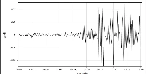
To solve the non stationary data, differencing process is needed. The result of Indonesian CPO export value data plot with first differences is in Figure 2:
Figure 2. Data Plot of Indonesian CPO Export Value With First Difference
From the data plot above, it show that the data of Indonesian CPO export value are stationary with the constant average of the first difference Indonesian CPO export data.
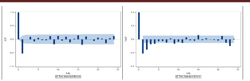
[image:5.595.170.427.511.641.2]Figure 3. The ACF and PACF Plot of Indonesian CPO Export Value with First Difference
[image:6.595.170.430.290.395.2]To make sure that the Indonesian CPO export value data is stationary, we use the Augmented Dickey Fuller (ADF) test. The result of this test in monthly data of Indonesian CPO Export Value can be seen in Table 1.
Table 1. ADF Test of Indonesian CPO Export Value Data with First Difference
Type Lags t-Statistic p-Value
Zero Mean 1 -18.9616 .0000
12 -5.22645 .0000
Single Mean 1 -18.9645 .0000
12 -5.53051 .0000
Trend 1 -18.9378 .0000
12 -5.58423 .0000
Table 1 show that the probability of all type of equation data (zero mean, single mean, and trend) in lag 1 and 12, is less than 5% alpha. Its mean that the null hypothesis is rejected and the data is stationary.
[image:6.595.92.504.531.715.2]After Indonesian CPO export value data with first differences already stationary, the next step is to get the value of p, d, and q to identification ARIMA(p,d,q) models. ACF and PACF plot value of Indonesian CPO exports with first differences, obtained some tentative ARIMA model, they are ARIMA (0,1,1), ARIMA (4,1,0) and ARIMA (4,1,1). After getting 3 tentative ARIMA model, the parameters will be estimated by ordinary least square method. Table 2 below shows the summary of the tentative ARIMA model parameter estimation.
Table 2. Parameter Estimation of Tentative ARIMA Model
No ARIMA Model Parameter AIC SBC Estimate p-value
1 ARIMA(0,1,1) C
MA(1)
41.49806 41.52941 6281108
-0.821410
.0428 .0000
2 ARIMA(4,1,0) C
AR(1) AR(2) AR(3) AR(4)
41.56466 41.64408 6284750
-0.830822 -0.610901 -0.319270 -0.169153
.2930 .0000 .0000 .0004 .0168
3 ARIMA(4,1,1) C
AR(1) AR(2) AR(3) AR(4) MA(1)
41.53976 41.63508 6759354
0.015584 0.085373 0.155315 0.029685 -0.892377
.0137 .8719 .3719 .0819 .7139 .0000
be seen from the p-value that less than 5% alpha. In the second equation, the parameter estimation is also significant, but the AIC and SBC values are greater than the first equation. While in the third equation, there is only one significant parameters estimation and the values of AIC and SBC is still greater than the first equation. So that, the best model is the ARIMA (0,1,1).
Overfitting is one way to check the model by fitting a model that is more common than tentative models. Overfitting of the ARIMA(0,1,1) will be performed with ARIMA (0,1,2) and ARIMA (1,1,1). The results of parameter estimation show that the ARIMA (0,1,1) remains the best model, because the parameter estimation in other models are not significant and its value of AIC and SBC are greater than the first model. So, the ARIMA(0,1,1) model is
Y =6281108+ 0.821410e + e .
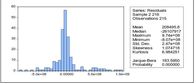
[image:7.595.129.471.317.462.2]After getting the ARIMA (0,1,1) as the best model, the next step is to analyze the residuals, includes examining normality, residuals white noise process, and homogeneity of variance. Normality examination is done by looking at residual plots and statistical tests Jarque-Bera. Figure 4 showed the histogram and the value of the Jarque-Bera statistics. From the histogram, it appears that the histogram does not resemble a symmetrical bell shape, which means that the residual is not the normal distribution. P-values Jarque-Bera statistic is less than 5% alpha, which also means that the residual is not the normal distribution.
Figure 4. Plot of Residual Normality and Jarque-Bera Statistics Tests
[image:7.595.108.489.538.614.2]To see the diagnostic of residuals white noise process, Ljung-Box Test Statistics (Q-statistic) are used. The test results showed that some of Ljung-Box statistic value at large lags are significant, so the residual is not a white noise process at large lags.
Table 3. The Results of Ljung-Box Test Statistics on Residual ARIMA (0,1,1)
Lags 1 6 12 18 24 30 36
ACF -.054 -.04 .091 -.05 .139 -.042 .074
PACF -.054 -.047 .123 -.076 .198 .021 .163
Q-Stat .6297 3.3514 11.828 21.544 36.848 48.802 63.223
Prob. .646 .377 .203 .034 .012 .002
[image:7.595.146.448.667.735.2]To see the diagnostic of residuals variance homogeneity, it can be determined by ARCH-Lagrange Multiplier test. The results of ARCH-LM test are shown in Table 4:
Table 4. The Results of ARCH-LM Statistics Tests on Residual ARIMA (0,1,1)
Lags F-statistic Obs*R-squared Prob. F Prob. Chi-Square
1 11.55459 11.06075 .0008 .0009
3 13.78602 35.16192 .0000 .0000
5 8.588122 36.51699 .0000 .0000
0 10 20 30 40 50 60
-5.0e+08 0.00000 5.0e+08 1.0e+09
Series: Residuals Sample 2 216 Observations 215
Mean 208495.8 Median -26107917 Maximum 9.74e+08 Minimum -8.07e+08 Std. Dev. 2.47e+08 Skewness 1.074718 Kurtosis 6.984251
From Table 4 above, it can be seen that the p-value for the Chi-Square on all the lag is smaller than 5% alpha, so the residuals variance is not homogeneous.
Log transformations
The ARIMA (0,1,1) obtained is still having variance heterogeneity problems, so the log transformation method will be performed on the data to overcome that problems and the new ARIMA model will be built. Data plots of log Indonesian CPO export value indicate that the data are not stationary. Likewise from the ACF plot looks down slowly, indicates that the data is not stationary.
The differencing process is used to overcome nonstationary of this data. The data plot, ACF plot, and PACF plot indicate that the log CPO export value data with first differences are already stationary. Using the ADF statistic test, the results also indicate that the log CPO export value data with first differences are already stationary.From the ACF plot and PACF plot, it can be seen that the ACF plot at first lag is significant, whereas the PACF plot at first lag and second lag are significant. So the tentative ARIMA (p,d,q) model are ARIMA (0,1,1), ARIMA (2,1,0) and ARIMA (2,1,1). From the three tentative ARIMA model, it can be seen that the ARIMA(2,1,1) is the best ARIMA model, because the value of AIC and SBC are smaller than others and the parameter estimation is significant.
Overfitting the ARIMA (2,1,1) will be compared with ARIMA (3,1,1) and ARIMA (2,1,2). The parameter estimation results are shown that from the three ARIMA models, only the ARIMA(2,1,1) that have a significant parameter estimation. So, the ARIMA (2,1,1) is still the best model. The ARIMA(2,1,1) model is
LogY =0.017890+0.347755LogY +0.142758LogY + 0.989811e + e .
By looking at the residual plots and statistical tests Jarque-Bera, it can be show that the residual is not the normal distribution. The results of Ljung-Box statistical tests show that, the residuals is a white noise process. The ARCH-LM statistical tests show that the p-value for the Chi-Square on all lag is greater than 5% alpha, so the residual variance is homogenous.
Building and studying the GARCH model
In the previous discussion, Model ARIMA (0,1,1) of the value of Indonesia's CPO export data has a heterogeneity of variance problem. By using a log transformation on the value of Indonesian CPO export data, heterogeneity of variance problem can be solved and obtained ARIMA (2,1,1). In this discussion, we will use the GARCH model to solve the heterogeneity of variance problem in ARIMA (0,1,1) model.
The first step is determining the order of the GARCH model. The determination of the order GARCH is starting from the smallest order, GARCH (1,1). The parameter estimation of GARCH (1,1) is used the maximum likelihood method. It showed that all parameter estimation are significant, so the GARCH (1,1) can be used. Overfitting is done to get a better GARCH model, namely with GARCH (1,2) and GARCH (2,1). In the second equation, all parameter estimation are significant, but the value of AIC and SBC are greater than the first equation. In the third equation, it appears that there is a parameter coefficient that not significant at the 5% alpha and AIC and SBC values are greater than the first equation. So, GARCH (1,1) model is the best model because it has the value of the smallest AIC and SBC. The GARCH(1,1) model is σ = ( 5.82 × 10 ) + 0.855671σ + 0.229671ϵ .
The examination of variance heterogeneity in the GARCH (1,1) is using the ARCH-LM statistic test. The results show that at all lags, the p-values for the Chi-Square are greater than alpha 5%, so the residual variance heterogeneity does not occured. The examination of residual normality can be seen from the histogram and Jarque-Bera statistical tests. The results show that the residual is not a normal distribution.
Indonesia's CPO export data and GARCH (1,1) Indonesian CPO export value data. The best model is a model that has a smaller value of MAE and MAPE. The results are in table below. It shows that the ARIMA(2,1,1) is better than the GARCH(1,1).
Table 5. The Results of ARCH-LM Statistic Test
Model MAE MAPE (%)
ARIMA(2,1,1) GARCH(1,1)
1.62E+08 3.09E+08
37.90131 69.50711
Forecasting
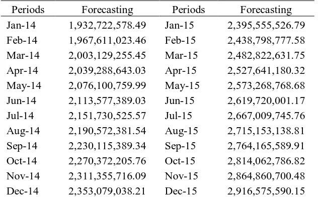
[image:9.595.141.457.227.423.2]The forecasting results of ARIMA(2,1,1) for 24 periods ahead are in the table 6: Table 6. The Results of Forecasting
Periods Forecasting Periods Forecasting
Jan-14 1,932,722,578.49 Jan-15 2,395,555,526.79
Feb-14 1,967,611,023.46 Feb-15 2,438,798,777.58
Mar-14 2,003,129,255.45 Mar-15 2,482,822,631.75
Apr-14 2,039,288,643.03 Apr-15 2,527,641,180.32
May-14 2,076,100,759.99 May-15 2,573,268,768.68
Jun-14 2,113,577,389.03 Jun-15 2,619,720,001.17
Jul-14 2,151,730,525.57 Jul-15 2,667,009,745.76
Aug-14 2,190,572,381.54 Aug-15 2,715,153,138.81
Sep-14 2,230,115,389.34 Sep-15 2,764,165,589.91
Oct-14 2,270,372,205.76 Oct-15 2,814,062,786.82
Nov-14 2,311,355,716.09 Nov-15 2,864,860,700.48
Dec-14 2,353,079,038.21 Dec-15 2,916,575,590.15
From the table above, it can be seen that the results of forecasting are increase at 24 periods ahead.
CONCLUTION
The problems of heterogeneity on ARIMA(0,1,1) of Indonesian CPO export value data can be solved with 2 methods. The first method is aARIMA model with a log transformation and the second is GARCH model. In the first method, the model that be built is more parsimonious than the second. Besides that, on the first method, the forecasting accuracy is better than the second. Both methods produce a homogeneous variance, but the second is better than the first. So, it can be concluded that ARIMA model is better than GARCH models. Based on the forecasting results, the future of Indonesian CPO export value will be better than present.
REFERENCES
Bollerslev, T. (1986). Generalized Autoregressive Conditional Heteroskedasticity. Journal of
Econometrics, 31, 307-327.
Cryer, J.D., Chan, K.S. (2008). Time Series Analysis with Application in R. New York, NY: Springer.
Department of Economic and Social Affairs Statistics Division. (1998). International
Merchandise Trade Statistics: Concepts and Definitions. New York, NY: United Nations.
Engle, R.F. (1982). Autoregressive Conditional Heteroscedasticity with Estimates of the Variance of United Kingdom Inflation. Econometrica, 50, 987-1007.
Engle, R.F., Bollerslev, T. (1986). Modelling the Persistence of Conditional Variances.
Econometric Reviews, 5(1), 1-50.
Hansen, K. (2008). Peramalan Produksi dan Ekspor Crude Palm Oil (CPO) Indonesia Serta
Implikasi Hasil Ramalan Terhadap Kebijakan. Bogor: Institut Pertanian Bogor.
Hariyadi, P. (2008). Mengenal Minyak Sawit dengan Beberapa Karakter Unggulnya. Jakarta: GAPKI.
Makridakis, S., Wheelwright, S.C., McGee, V.E. (1999). Metode dan Aplikasi Peramalan, Edisi
Kedua, Jilid 1. Andriyanto, U.S., Basith, A., translators. Jakarta: Erlangga. Translation of:
Forecasting, 2nd Edition.
Wei, W.W.S. (2006). Time Series Analysis, Univariate and Multivariate Methods, Second
Edition. New York, NY: Pearson Education, Inc.