The Impact of Obesity on Wages
John Cawley
a b s t r a c t
Previous studies of the relationship between body weight and wages have found mixed results. This paper uses a larger data set and several regres-sion strategies in an attempt to generate more consistent estimates of the effect of weight on wages. Differences across gender, race, and ethnicity are explored.
This paper nds that weight lowers wages for white females; OLS esti-mates indicate that a difference in weight of two standard deviations (roughly 65 pounds) is associated with a difference in wages of 9 percent. In absolute value, this is equivalent to the wage effect of roughly one and a half years of education or three years of work experience. Negative cor-relations between weight and wages observed for other gender-ethnic groups appear to be due to unobserved heterogeneity.
I. Introduction
Several previous studies have found, among females, a negative cor-relation between body weight and wages.1There exist three broad categories of ex-planations for this nding. The rst explanation is that obesity lowers wages; for example, by lowering productivity or because of workplace discrimination. The sec-ond is that low wages cause obesity. This would be true if poorer people consume
John Cawley is an assistant professor of policy analysis and management at Cornell University. For their helpful comments, he thanks Susan Averett, Gary Becker, John Bound, Charlie Brown, Rachel Dunifon, Michael Grossman, James Heckman, Sanders Korenman, Darius Lakdawalla, Helen Levy, Will Manning, David Meltzer, Tomas Philipson, Chris Ruhm, seminar participants, and two anonymous referees. The author thanks Justine Lynge for editorial assistance. The data used in this article can be obtained beginning October 2004 through September 2007 from John Cawley, 134 MVR Hall, Depart-ment of Policy Analysis and ManageDepart-ment, Ithaca, NY 14853-4401. Email: jhc38@cornell.edu. [Submitted September 2000; accepted January 2003]
ISSN 022-166X; E-ISSN 1548-8004Ó2004 by the Board of Regents of the University of Wisconsin System 1. See, for example, Register and Williams (1990), Averett and Korenman (1996), and Pagan and Davila (1997).
452 The Journal of Human Resources
cheaper, more fattening, foods. The third category of explanations is that unobserved variables cause both obesity and low wages. This paper uses several econometric methods in an effort to determine which of these three explanations is responsible for the correlation between weight and wages. Differences in the correlation between weight and wages across gender, race, and ethnicity are explored. The question of how obesity correlates with labor market outcomes, and why, is important in part because the prevalence of obesity in the United States has risen dramatically in recent years, from 15 percent during 1976– 80 to 30.9 percent during 1999– 2000.2
The outline of this paper is as follows. Section II presents a basic model of weight and wages. Section III discusses the methods and related literature in the context of the model. The data used in this paper are described in Section IV. Empirical results are presented in Section V.
II. A Model of Weight and Wages
Assume that wagesWand Body Mass Index (or BMI)3Bhave the following relationship for individual iat timet:
(1) lnWit5Bitb1Xitg1eit
In Equation 1, X is a vector of variables that affect wages (such as measures of human capital) andeis the residual.
If BMI is strictly exogenous then an OLS estimate of bcan be interpreted as a consistent estimate of the true effect of BMI on log wages. However, research in behavioral genetics suggests that roughly half of the variation in BMI is due to nongenetic factors such as individual choices and environment.4In addition, obesity may be inuenced by wages, especially for adult females.5Each of these ndings suggests that BMI may be endogenous.
To classify the sources of potential endogeneity in weight, the wage residual in Equation 1 can be decomposed as having a genetic component GW, a nongenetic
component NGW, and a residualnthat is i.i.d. over individuals and time.
(2) eit 5GWit 1NGWit 1nit
BMI may in turn be affected by wages and personal characteristics.
(3) Bit5Xitg1Wita1Zitf1GBit 1NGBit1xit
2. Flegal et al. (2002).
3. BMI is calculated as weight in kilograms divided by height in meters squared. BMI is the standard measure of fatness in epidemiology and medicine (U. S. Department of Health and Human Services, 2001). For example, BMI is used to classify individuals as overweight and obese by the U. S. National Institutes of Health, the World Health Organization, and the International Obesity Task Force; see Flegal et al. (1998).
4. Genes explain roughly half of the cross-sectional and temporal variation in individual weight (see, for example, Comuzzie and Allison, 1998). Individual environment and choices appear to be responsible for the other half of variation.
Cawley 453
In Equation 3, X is the same vector of variables that affect wages,W represents wages,Zis a vector of variables that affect BMI but do not directly affect wages, GB represents the inuence of genetics on BMI, NGB represents the inuence of
nongenetic factors (such as an individual’s choices, upbringing, and culture) on BMI. Residual BMI is represented byx. The variables on the right-hand side of Equation 3 indicate the potential pitfalls of an OLS estimation of Equation 1: current wages may affect BMI (ifa ¹0), genetic factors that inuence BMI (GB) may be correlated
with genetic factors that affect wages (GW), and nongenetic factors that inuence
BMI (NGB) may be correlated with nongenetic factors that affect wages (NGW).
Each of these scenarios implies that the OLS assumption thatBis uncorrelated with
ein Equation 1 is violated and that an OLS estimate ofbis biased.
III. Methods and Previous Studies
Several papers have studied the relationship between body weight and either wages or income,6but this section reviews only those that took steps to deal with the potential endogeneity of weight when estimating the effect of weight on wages.
In the previous literature, three strategies have been used to adjust for the likelihood that weight is endogenous. The rst is to replaceBwith a lagged value ofB. This strategy is based on the assumption that lagged weight is uncorrelated with the current wage residual:Bit2t eit, which assumes no serial correlation in the wage residuals
for the two periods:eit2t eit. While this strategy will remove any contemporaneous
effect of wages on weight, it does not deal with the problem that the genetic and nongenetic components of lagged weight (GB
it2tandNGBit2t) may be correlated with
the genetic and nongenetic components of current wages (GW
it andNGWit).
Gortmaker et al. (1993), Sargent and Blanchower (1995), and Averett and Koren-man (1996) regressed current income or wages on measures of body weight from seven years earlier. Each found that the income or wages of young females was lower if they had been overweight or obese in the past. Each study also found little if any evidence of a difference in income or wages for males based on weight status seven years earlier.
The second strategy used to deal with the endogeneity of weight is to estimate Equation 1 after taking differences with another individual with highly correlated genes (either a same-sex sibling or twin). Based on Equation 3, the differenced re-gressor of interest is:
B1t2B2t5(X1t 2X2t)g1(W1t2W2t)a1(Z1t2Z2t)f 1(GB
1t2GB2t)1(NGB1t2NGB2t)1(x1t2x2t)
The differencing strategy assumes that all unobservable heterogeneity is constant within pairs (that is, thatG15G2andNG15NG2) so that all relevant unobserved heterogeneity is differenced away. This strategy also assumes that wages do not
454 The Journal of Human Resources
inuence weight (a5 0), so that the differenced weight variable is uncorrelated with the differenced wage residual (B1t 2B2t) (e1t2e2t).
Averett and Korenman (1996), in addition to using lagged values of weight, differ-ence between siblings. In taking this differdiffer-ence, they eliminate the variance in weight attributable to shared genes or shared environment. However, after differencing they are still left with: a) the variance in weight attributable to genes unshared by siblings since G1 ¹ G2 within sibling pairs, and b) the variance in weight attributable to nongenetic factors unshared by siblings sinceNG1¹NG2within sibling pairs. The coefcients on weight estimated by the sibling-differencing procedure of Averett and Korenman are not statistically signicant, which is attributable in part to their small sample of siblings (288 sister pairs and 570 brother pairs).
Behrman and Rosenzweig (2001) examine the relationship between BMI and wages among females in the Minnesota Twins Registry. The drawback of this data is its relatively small sample size; even the OLS coefcient on BMI is not statistically signicant if they control for schooling and work experience (N51,518). The au-thors estimate a regression differencing within 808 monozygotic (MZ) twin pairs; the coefcient on weight is not statistically signicant.
The third strategy used to deal with the endogeneity of weight is to use variables Z as instruments in IV estimation under the assumption that Zit eit. Pagan and
Davila (1997) nd using OLS that obese females earn less than their more slender counterparts and seek to determine whether their OLS estimate is biased. Using a Hausman specication test, they fail to reject the hypothesis that weight is uncorre-lated with the error term of the wage equation. However, their test is called into question because their instruments (family poverty level, health limitations, and indi-cator variables about self-esteem) are likely correlated with the error term in the wage equation. Given that their IV estimation likely suffers the same kind of bias as OLS, it is not surprising that, through their Hausman test, they fail to reject the hypothesis that OLS and IV coefcients are equal.
Behrman and Rosenzweig (2001), after removing the variation common between MZ twins, seek to remove any remaining endogeneity through IV, using lagged weight as an instrument. Their IV coefcient on BMI is not statistically signicant. This paper will estimate the effect of weight on wages using OLS and each of the three strategies described above to deal with the potential endogeneity of weight. This paper uses a larger data set to produce more precise estimates and also seeks to use better instruments to generate a more consistent IV estimate. An additional innovation of this paper is to correct the self-reported measures of weight and height for reporting error.
IV. Data: National Longitudinal Survey of Youth
Cawley 455
At the baseline of the NLSY, respondents were asked to report their race or eth-nicity, which the NLSY simplied into three groups: black, Hispanic, and nonblack/ nonHispanic. For the sake of brevity, the last group is referred to as white throughout this paper, although it is a heterogeneous group.
The NLSY recorded the self-reported weight of respondents in 1981, 1982, 1985, 1986, 1988, 1989, 1990, 1992, 1993, 1994, 1996, 1998, and 2000. Data from these 13 years were pooled to create the sample used in this paper. Reported height was recorded in 1981, 1982, and 1985; given that respondents were between the ages of 20 and 27 in 1985, height in 1985 was assumed to be the respondents’ adult height. These self-reports of weight and height include some degree of reporting error, which may bias coefcient estimates.7In order to correct for this reporting error, true height and weight in the NLSY are predicted using information on the relation-ship between true and reported values in the Third National Health and Nutrition Examination Survey (NHANES III)8and using the method outlined in Lee and Sep-anski (1995) and Bound et al. (2002). Separately by race and gender, actual weight was regressed on reported weight and its square. This process was repeated for height. Self-reported height and weight in the NLSY are then multiplied by the coef-cients on the reported values associated with the correct race-gender group in the NHANES III. The tted values of weight and height, corrected for reporting error, are used throughout the paper.9
This paper uses three measures of body weight: (1) body mass index (BMI); (2) weight in pounds (controlling for height in inches); and (3) indicator variables for the clinical classications underweight, overweight, and obese, where the excluded category is healthy weight.10
Weight tends to rise with age. In order to distinguish the effects of weight from those of age and time, linear measures of age and time are included as regressors in the log wage regressions.
Weight also may be affected by current or recent pregnancy. For this reason, females who are pregnant at the time that they report their body weight are dropped from the sample.11To control for effects of recent pregnancy, the set of regressors includes the age of a woman’s youngest child and the total number of children to whom she has given birth.
The following variables are included as regressors in order to control for differ-ences in human capital: general intelligence (which is a measure of cognitive ability derived from the ten Armed Services Vocational Aptitude Battery tests administered
7. See Judge et al. (1985).
8. Third National Health and Nutrition Examination Survey (NHANES III) conducted in 1988– 94, sur-veyed a nationally representative sample of 33,994 persons aged 2 months and older; 31,311 of those respondents also underwent physical examinations.
9. An appendix detailing this correction for reporting error is available from the author upon request. 10. The U. S. National Institutes of Health classies BMI as follows: below 18.5 is underweight, between 18.5 and 25 is healthy, between 25 and 30 is overweight and over 30 is obese. See U. S. National Institutes of Health (1998) and Epstein and Higgins (1992).
456 The Journal of Human Resources
in 1980),12highest grade completed, mother’s highest grade completed, and father’s highest grade completed. The following regressors are included to control for charac-teristics of employment: years of actual work experience (dened as weeks of re-ported actual work experience divided by 50), job tenure, and indicator variables for whether the respondent’s occupation is white collar or blue collar,13current school enrollment, county unemployment rate, and whether the respondent’s job is part-time (dened as less than 20 hours per week). The set of regressors also includes age, year, and indicator variables for marital status and region of residence. Indicator variables for missing data associated with each regressor, except the weight vari-ables, are also included.
In each year, the NLSY calculates the hourly wage earned by the respondent at his or her primary job. Outliers in wage are recoded; if the hourly wage is less than $1 an hour, it is recoded to $1 and if the hourly wage exceeds $500 an hour, it is recoded to $500.14
Gortmaker et al. (1993) studied 1988 earnings data from the NLSY and Pagan and Davila (1997) studied 1989 data from the same source. The primary sample used by Averett and Korenman (1996) is also a single year of data (1988) from the NLSY, and in an appendix they present results for three years of data (1988– 90) pooled. This paper also studies the NLSY but pools all 13 years that contain weight data.
Appendix Tables A1 and A2 provide summary statistics for the samples of females and males.
NLSY sample weights are used in all estimations described in this paper.T-statistics reported for OLS and IV regressions reect robust standard errors that are calculated with clustering by individual to account for correlations in the error terms of each individual over time.
V. Empirical Results
The hypotheses that all coefcients are equal across race/ethnic groups, and that the coefcients on BMI are equal across race/ethnic groups, were tested. For both males and females, each hypothesis was rejected at the 5 percent signicance level, so regressions are estimated separately by race and gender. Results for women are presented in Table 1 and those for men are presented in Table 2.15
12. See Jensen (1987) for a full description of this measure of cognitive ability.
13. All occupations are classied as either white collar or blue collar using Census codes for occupation. White collar workers are those working in sectors described by the U. S. Census as Professional, Technical, or Kindred Workers, NonFarm Managers and Administrators, Sales Workers, and Clerical and Unskilled Workers.
14. As a result, 634 person-year observations are bottom-coded and 55 person-year observations are top-coded.
Cawley 457
Columns 1, 4, and 7 of Table 1 indicate that, for each group of females, both BMI and weight in pounds have negative and statistically signicant OLS coef-cients. The point estimate is largest for white females and smallest for black females. An increase of two standard deviations (64 pounds) from the mean weight in pounds among white females is associated with a decrease in wages of 9 percent, which is roughly equal in magnitude to the difference associated with 1.5 years of education, or three years of work experience. In contrast, for black females, an increase in weight of two standard deviations (79 pounds) from the mean is associated with a decrease in wages of 4.7 percent, and the same two standard deviation increase for Hispanic females (62 pounds) is associated with a decrease in wages of 6.8 percent. Columns 1, 4, and 7 of Table 2 indicate that the signs and magnitudes of the OLS coefcients on weight for males vary by ethnic group. For white males, the coefcients on BMI and weight in pounds are not signicantly different from zero. For black males, higher body weight is associated withhigherwages; an increase in weight of two stan-dard deviations (70 pounds) from the mean weight in pounds is associated with a 4.2 percent increase in wages. The coefcients on weight for Hispanic males resemble those for females: negative and statistically signicant. Among Hispanic males, an increase in weight of two standard deviations (73.5 pounds) from the mean weight in pounds is associated with a decrease in wages of 8.1 percent, which is similar in magnitude to the wage effect of 2.5 years of education or 4.5 years of work experience.
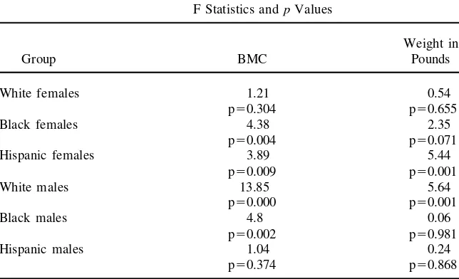
Equation 1 assumes that log wages are linear in BMI (or weight in pounds). Table 3, which contains the results of RESET tests for linearity,16 indicates that at a 5 percent signicance level, the hypothesis of linearity of wages in BMI is rejected for black females, Hispanic females, white males, and black males, but that it is impossible to reject the hypothesis of linearity for white females and Hispanic males. At the same signicance level, the hypothesis of linearity of wages in weight in pounds is rejected for Hispanic females and white males but cannot be rejected for any other group. Given this evidence that wages may be nonlinear in weight for certain measures of weight and certain race-ethnic groups, models are also estimated using indicator variables for clinical weight classication.
Columns 1, 4, and 7 of Tables 1 and 2 also present the OLS coefcients on the indicator variables for clinical weight classication. Among white females, there is no detectable wage differential between those who are underweight relative to those of healthy weight, but those who are overweight earn 4.5 percent less than those of healthy weight, and those who are obese earn, on average, 11.9 percent less than those of healthy weight— this is roughly equal to the effect of 1.8 years of education or 3.8 years of work experience.
Among black and Hispanic females, the OLS coefcients indicate that those who are overweight earn no less than those of healthy weight, while those who are obese earn roughly 6–8 percent less. Black females are the only females for whom the underweight earn less than those of healthy weight.
The pattern of log wages over weight classication is an inverted U shape for white males. In Table 2, the point estimate of the coefcient on the indicator for
sample. The adjustment also had very little effect on the magnitude of the coefcients on weight, so only results without the Heckman selection correction are presented in this paper.
458
The
Journa
l
of
Hum
an
Re
so
ur
ce
s
Table 1
Coefcients and t-Statistics from Log Wage Regressions for Females
White Females Black Females Hispanic Females
OLS OLS Fixed OLS OLS Fixed OLS OLS with Fixed
with Lag Effects with Lag Effects Lag Weight Effects
Weight Weight
Column Number 1 2 3 4 5 6 7 8 9
BMI 20.008 20.008 20.007 20.004 20.005 20.0001 20.006 20.006 20.003 (27.01) (24.62) (25.73) (23.20) (23.09) (20.11) (23.31) (22.73) (21.19) Weight in pounds 20.0014 20.0014 20.0012 20.0006 20.0009 0.0001 20.0011 20.0012 20.0005
(26.98) (24.73) (25.65) (23.16) (23.00) (0.15) (23.35) (22.77) (21.26) Underweight 20.01 0.019 20.011 20.056 20.021 20.084 20.042 20.071 0.028 (20.53) (0.81) (20.75) (22.18) (20.99) (23.61) (21.17) (21.62) (0.79) Overweight 20.045 20.080 20.016 20.011 20.080 0.018 20.015 20.039 0.006 (23.52) (24.35) (21.63) (20.75) (24.35) (1.48) (20.75) (21.50) (0.39) Obese 20.119 20.089 20.087 20.061 20.077 0.002 20.082 20.098 20.02
(26.76) (23.35) (25.88) (23.31) (22.99) (0.12) (23.22) (22.82) (20.83) Number of observations 25,843 9,972 25,843 11,742 9,972 11,742 7,533 3,092 7,533
Notes:
1) Data: NLSY females
2) One of three measures of weight is used: BMI, weight in pounds (controlling for height in inches) or the three indicator variables for clinical weight classication: underweight, overweight, and obese (where healthy weight is the excluded category).
3) For BMI and weight in pounds, coefcients andtstatistics are listed. For indicators of clinical weight classication, the percent change in log wages associated with a change in the indicator variable from 0 to 1 andtstatistics are listed.
C
aw
le
y
459
Table 2
Coefcients and t-Statistics from Log Wage Regressions for Males
White Males Black Males Hispanic Males
OLS OLS Fixed OLS OLS Fixed OLS OLS with Fixed
with Lag Effects with Lag Effects Lag Weight Effects
Weight Weight
Column Number 1 2 3 4 5 6 7 8 9
BMI 20.001 20.003 20.0001 0.004 0.005 0.003 20.007 20.009 20.002
(20.83) (21.54) (20.21) (2.19) (2.04) (1.96) (23.12) (23.15) (21.03) Weight in pounds 20.0002 0.0005 0.0001 0.0006 0.0007 0.0005 20.0011 20.001 20.0003
(21.01) (21.68) (0.07) (2.21) (2.06) (1.96) (23.47) (23.18) (20.90) Underweight 20.14 0.005 20.035 20.099 20.046 0.013 0.029 0.107 20.005 (23.05) (0.07) (21.12) (22.75) (20.70) (0.28) (0.44) (1.13) (20.12)
Overweight 0.039 0.016 0.022 0.031 0.019 0.014 20.025 20.021 0.018
(3.04) (1.05) (2.63) (1.87) (0.94) (1.14) (21.13) (20.82) (1.15)
Obese 20.033 20.075 0.013 0.043 0.042 0.031 20.066 20.100 0.023
(21.73) (23.05) (0.89) (1.80) (1.29) (1.64) (22.21) (22.41) (0.91) Number of observations 29,410 12,410 29,410 13,414 6,128 13,414 9,070 4,079 9,070
Notes:
1) Data: NLSY males.
2) One of three measures of weight is used: BMI, weight in pounds (controlling for height in inches) or the three indicator variables for clinical weight classication: underweight, overweight, and obese (where healthy weight is the excluded category).
3) For BMI and weight in pounds, coefcients andtstatistics are listed. For indicators of clinical weight calssication, the percent change in log wages associated with a change in the indicator variable from 0 to 1 andtstatistics are listed.
460 The Journal of Human Resources
Table 3 Test of Linearity
F Statistics andpValues
Weight in
Group BMC Pounds
White females 1.21 0.54
p50.304 p50.655
Black females 4.38 2.35
p50.004 p50.071
Hispanic females 3.89 5.44
p50.009 p50.001
White males 13.85 5.64
p50.000 p50.001
Black males 4.8 0.06
p50.002 p50.981
Hispanic males 1.04 0.24
p50.374 p50.868
Notes: 1) Data: NLSY.
2)Fstatistics are associated with Thursby and Schmidt (1977) tests of linearity; specically, with the hypothesis that the coefcients on the weight measure to the second, third, and fourth powers are jointly equal to zero.
underweight is negative, that for overweight is positive, and that for obese is nega-tive. While the OLS coefcients on both BMI and weight in pounds were positive and signicant for black males, the OLS coefcients on the indicator variables for weight classication indicate that this is due to underweight black men earning less than healthy weight black men, not due to overweight and obese black men earning more than healthy weight black men (though the point estimates of the coefcients on overweight and obese are positive).
The OLS results for Hispanic males resemble those for Hispanic females; the coefcient on underweight is not statistically signicant, while that on obese is statis-tically signicant and negative.
Averett and Korenman (1996) report a coefcient on obesity for white females that is strikingly similar:20.12 compared with20.119 found in this paper.17Their coefcient on obesity for black females is also virtually identical but is not statisti-cally signicant.
The OLS estimates suggest that, in general, heavier females of each ethnic group and heavier Hispanic males tend to earn less than members of the same group of
Cawley 461
healthy weight. However, as mentioned earlier, OLS estimates of the coefcient on weight in Equation 1 are questionable because there may exist reverse causality; that is, heavier people may tend to earn less because low wages result in weight gain. The previous literature tried to eliminate such effects by substituting a lagged value of weight for its contemporaneous value. Each of the three papers in the previ-ous literature to use this strategy (Gortmaker et al., 1993; Sargent and Blanchower, 1995; and Averett and Korenman, 1996) used a lag of seven years, so to facilitate comparisons this paper will follow that convention. Columns 2, 5, and 8 in Tables 1 and 2 present OLS results using a measure of weight lagged seven years. The point estimates of the lagged measures of BMI and weight in pounds are, in general, similar to those on current weight. The smaller sample sizes in the lagged regressions result in higher standard errors, so in some cases the coefcients are not statistically signicant in a lagged regression while a similar point estimate is signicant in the contemporaneous regression.
The high degree of similarity between the point estimates on linear measures of weight in the lagged and contemporaneous OLS regressions is consistent with either of two hypotheses: either (a) current wages have little impact on current weight; or (b) current wages do affect current weight, but there is such high serial correlation in both wages and weight that when even distant BMI is used as a regressor, the effect of wages on weight is measured just as strongly.
Differences in coefcients on lagged and contemporaneous values of weight are greater in the regressions using indicator variables for weight classication; for ex-ample, the indicator for lagged underweight status has a considerably smaller point estimate than that for contemporary underweight status for white and black men. Furthermore, lagged (but not contemporaneous) obesity is statistically signicant and negative for white males. With the exception of white females, the coefcients on lagged obesity tend to be larger in absolute than those on contemporaneous obe-sity; this is consistent with the results of Averett and Korenman (1996).18
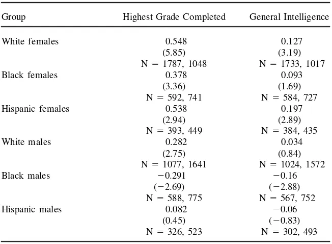
The strategy of using lagged weight does not address the issue of time-invariant heterogeneity on both weight and wages. It is impossible to test for the presence of unobserved heterogeneity, but a comparison across weight groups of important observed variables that are known to affect wages can be suggestive. Table 4 lists the average intelligence test score and education of those who according to clinical classications are underweight or healthy weight compared to those who are over-weight or obese, within each gender-ethnic group. T-statistics associated with the hypothesis that the difference between the group means is zero appear in parentheses. Table 4 indicates that for each group of females, those in the lighter group have on average more years of education and higher test scores than those who are in the heavier group. The results for males are again very different from those for females; of four comparisons for white males and Hispanic males, only for the education of white males is the difference statistically signicant, with lighter individuals having on average a higher value of the human capital measure. In contrast, among black males, the difference is statistically signicant and negative for both education and intelligence test scores—that is, black males who are overweight or obese tend to have on averagehighereducation and intelligence scores than black males who are
462 The Journal of Human Resources
Table 4
Difference in Unconditional Means between (Underweight and Healthy Weight) and (Overweight and Obese)
Group Highest Grade Completed General Intelligence
White females 0.548 0.127
(5.85) (3.19)
N51787, 1048 N 51733, 1017
Black females 0.378 0.093
(3.36) (1.69)
N5592, 741 N5584, 727
Hispanic females 0.538 0.197
(2.94) (2.89)
N5393, 449 N5384, 435
White males 0.282 0.034
(2.75) (0.84)
N51077, 1641 N 51024, 1572
Black males 20.291 20.16
(22.69) (22.88)
N5588, 775 N 5567, 752
Hispanic males 0.082 20.06
(0.45) (20.83)
N5326, 523 N5302, 493
Notes: 1) Data: NLSY.
2) Includes one observation of each individual, observed between the ages of 28 and 32.
3) Listed is the difference in means between the lighter group and the heavier group, thetstatistic associated with the hypothesis that the two means are equal, and the number of observations in the two groups. A positive difference in the means indicates that the lighter group has a higher mean than the heavier group.
lighter. This correlation suggests that unobserved heterogeneity is the reason that black males were the only group with a positive correlation between wages and either BMI or weight in pounds. If unobserved variables that affect wages are correlated with weight in the same way education and intelligence test scores are correlated with weight, then omitted variable bias in OLS estimates ofbwill generate spurious results that imply that weight lowers wages for females and weight raises wages for black men.
These ndings for females are consistent with those of Sargent and Blanchower (1994), who nd that girls (but not boys) obese at age 16 performed worse than those not obese at age 16 on math and reading tests in later years. They also found that both men and women who had been obese at age 16 ended up with fewer years of schooling than those not obese at age 16. Similarly, Gortmaker et al. (1993) nd that women, but not men, who were overweight in 1981 had less education in 1988 compared to those who had not been overweight in 1981.
Cawley 463
previous literature took differences between siblings or twins, this paper exploits the longitudinal nature of the NLSY data to eliminate individual-specic xed effects. Assuming that the inuence of genes and nongenetic factors is constant over time, the individual xed-effects method eliminates more variation due to unobserved non-genetic factors than does differencing between either siblings or twins, and will elim-inate just as much of the variation due to genes as differencing between MZ twins (which is more than is eliminated by differencing between nontwin siblings).
Columns 3, 6, and 9 of Tables 1 and 2 report estimates from xed-effects regres-sions. The most dramatic difference is that the negative coefcients on BMI and weight in pounds are much smaller and no longer statistically signicant for black females, Hispanic females, and Hispanic males. This suggests that the OLS results for these groups are driven largely by unobserved time-invariant heterogeneity.
The coefcients on BMI and weight in pounds are virtually unchanged for white females. The xed-effects coefcients for black males are smaller than those from OLS and are just barely statistically signicant at a 5 percent level. So far, the nding that heavier white females earn less and heavier black males earn more is robust.
Linearity of wages in weight was rejected for black and Hispanic females, as well as for white males. For these three groups, the small xed-effects point estimates could be due to differencing across a nonlinear function. Columns 3, 6, and 9 of Tables 1 and 2 also list the xed-effects estimates of coefcients on indicator vari-ables for weight classication. Each of the coefcients on clinical weight classica-tion is not statistically signicant for Hispanic females. However, the coefcient on the indicator variable on underweight is statistically signicant and negative for black females, and the indicator for overweight is statistically signicant and positive for white males.19 No xed-effects coefcient on weight classication is statistically signicant for black men. It is also noteworthy that the xed-effects coefcient on obesity is statistically signicant and negative for white females, which is consistent with the results from both the OLS with current weight and the OLS with lagged weight regressions. These results suggest that the negative correlations between weight and wages observed for black females, Hispanic females, and Hispanic males are due to unobserved time-invariant heterogeneity; once time-invariant heterogene-ity is eliminated, negative correlations between weight and wages disappear. In con-trast, the negative correlation between weight and wages persists for white females. Behrman and Rosenzweig (2001) nd no statistically signicant relationship be-tween BMI and wages once they difference within female MZ twins. However, the small size of their sample (N 5808) may partly explain their failure to reject the hypothesis of no effect of weight on wages. For both males and females (with blacks, whites, and Hispanics pooled), Averett and Korenman (1996) nd negative but not statistically signicant coefcients on indicator variables for weight status in their within-sibling regressions.20 However, their failure to reject the hypothesis of no
19. The nding that the coefcient on the indicator for overweight is statistically signicant for white males in the OLS with current weight and xed-effects regressions is consistent with McLean and Moon (1980), which nds in 1973 data from the National Longitudinal Survey of Mature Men that overweight middle-aged men earn more than lighter men of the same age; they attribute this to a “portly banker” effect; that in certain groups girth is a signal of power or strength that commands respect.
464 The Journal of Human Resources
effect of weight on wages may also be partly due to their small samples of siblings: 288 sisters and 570 brothers.
A xed-effects strategy improves on OLS but is not ideal because unobserved factors inuencing both weight and wages may vary over time. To deal with this problem, this paper turns to the method of instrumental variables. If one can identify a set of instru-mentsZthat are correlated with BMI but not withe, the error term in wages, then one can calculate an instrumental variables estimate of b. This paper uses an instrument correlated with the genetic variation in weight (GB): the BMI of a sibling, controlling
for the age and gender of the sibling. The BMI of a sibling (BS) is assumed to be
correlated with the sibling’s personal characteristics, wages, and genes:
Bst5Xstg1Wsta1GBst1NGBst1xst
The identifying assumption has two parts. The rst is that the BMI of a sibling is strongly correlated with the BMI of the respondent. Siblings with the same parents are expected to share half of their genes, ensuring a high correlation between the siblings’ genetic variation in weightGB
SandGBi. Given that about half of the variation
in weight is genetic in origin,21 this ensures a strong correlation between sibling weights BSandBi.
The second part of the identifying assumption is that the weight of a sibling is uncorrelated with the respondent’s wage residual. One might be concerned that the nongenetic variation in sibling weight NGB
S is correlated with the respondent’s wage
residual through the nongenetic variation in the respondent’s wageNGWif both are,
in part, determined by habits learned in the parents’ household. However, studies have been unable to detect any effect of common household environment on body weight. Adoption studies have consistently found that the correlation in BMI between a child and its biological parents is the same for adoptees and natural children; that is, all of the correlation in weight can be attributed to shared genes and there is no effect attribut-able to shared family environment. This has been found for BMI,22weight class,23and even body silhouette.24Consistent with these ndings, studies have been unable to reject the hypotheses that the correlations in weight, weight for height, and skinfold measures between unrelated adopted siblings are equal to zero.25 Studies of twins reared apart also nd no effect of a shared family environment on BMI; there is no signicant difference between the correlation in weight of twins reared together and twins reared apart, nor is the correlation affected by age at separation or the similarity of separate rearing environments.26Grilo and Pogue-Geile (1991), a comprehensive review of studies of the genetic and environmental inuences on weight and obesity, conclude that “. . . only environmental experiences that are not shared among family members appear to be important. In contrast, experiences that are shared among family members appear largely irrelevant in determining individual differences in weight and obesity.”27It is not possible to prove the null hypothesis of no effect of household
21. Comuzzie and Allison (1998). 22. Vogler et al. (1995). 23. Stunkard et al. (1986). 24. Sorensen and Stunkard (1993). 25. Grilo and Pogue-Geile (1991).
Cawley 465
environment on body weight; the repeated failure to reject the null hypothesis is the strongest evidence that will ever be available. In addition, decades may have passed since the NLSY siblings lived in the same household, presumably weakening any household environment effect that ever did exist.
Alternately, one might be concerned that the genetic variation in sibling weight GB
S is correlated with the respondent’s wage residual through genetic variation in
respondent’s wage GW. For this to be true, the genes that determine weight and
any genes that determine wages would have to be either the same or bundled in transmission.
While it is impossible to prove the null hypothesis that sibling BMI is uncorrelated with the residual in the respondent’s wage equation, it can be informative to examine whether sibling weight is correlated with observables that are believed to be related to unobserved factors that affect the wage residual. To this end, years of education and the intelligence test score of the respondent were regressed on the set of instru-ments (sibling weight, sibling age, and sibling gender) and the other regressors (ex-cept weight) from the wage regressions. While this is not a denitive test, if the instruments are correlated with these observables it would suggest that eitherGB
Sor NGB
S is correlated with the respondent’s wage residual and would cast doubt on the
instruments’ validity. However, the suggestive evidence from this test is consistent with the identifying assumption; in only one of 12 regressions (two outcomes by six race-gender groups) was the set of instruments signicant at the 10 percent level—roughly what one would expect by chance.
A different observation of BMI from the same sibling is used as an instrument for each observation of respondent weight. Results from the rst-stage regression conrm that sibling weight is a powerful instrument for respondent weight. TheF statistic associated with the hypothesis that the rst-stage coefcients on the instru-ments are jointly equal to zero was over 30 for white males and females, over 20 for black males and females, and was roughly 8 for Hispanic females and roughly 20 for Hispanic males; for ve of the six groups this F statistic far exceeds the minimum F statistic of 10 suggested by Staiger and Stock (1997). For each race-gender group, the partial R-squared contributed by the instruments in the rst stage is greater than 0.04.
IV coefcients on BMI and weight in pounds are presented in Columns 2, 4, and 6 of Tables 5 and 6. (Columns 1, 3, and 5 in those tables present, for the sake of comparison, OLS coefcients estimated using the IV sample.) IV has not been used to estimate coefcients on the indicator variables for clinical weight classication because there are three indicators for weight classications in a single regression but only one instrument.
endoge-466
The
Journa
l
of
Hum
an
Re
so
ur
ce
s
Table 5
IV Coefcients and t-Statistics from Log Wage Regressions for Females
White Females Black Females Hispanic Females
OLS Using IV OLS Using IV OLS Using IV
Sample IV Sample IV Sample IV
Column Number 1 2 3 4 5 6
BMI 20.010 20.017 20.003 20.002 20.006 20.012
(26.10) (23.38) (22.13) (20.32) (22.35) (20.99)
F532.77 F520.36 F58.29
Weight in pounds 20.0016 20.0028 20.0006 20.0003 20.0012 20.0023
(25.97) (23.40) (22.05) (20.31) (22.44) (21.02)
F532.79 F520.08 F58.48
Number of observations 10,800 10,800 5,651 5,651 3,035 3,035
Notes:
1) Data: NLSY females.
2) One of two measures of weight is used: BMI or weight in pounds (controlling for height in inches). 3) Coefcients andt-statistics are listed.
4) Other regressors include: Number of children ever born, age of youngest child, general intelligence, highest grade completed, mother’s highest grade completed, father’s highest grade completed, years of actual work experience, job tenure, age, year, and indicator variables for marital status, county unemployment rate, current school enrollment, part-time job, white collar job, and region of residence.
C
aw
le
y
467
Table 6
IV Coefcients and t-Statistics from Log Wage Regressions for Males
White Males Black Males Hispanic Males
OLS Using OLS Using OLS Using
IV Sample IV IV Sample IV IV Sample IV
Column Number 1 2 3 4 5 6
BMI 20.001 20.013 0.006 20.003 20.006 20.009
(20.45) (21.57) (2.22) (20.38) (22.5) (21.25)
F531.32 F526.16 F521.21
Weight in pounds 20.0002 20.0021 0.0009 20.0004 20.0010 20.0018
(20.54) (21.72) (2.34) (20.37) (22.67) (21.62)
F529.84 F526.34 F520.07
Number of observations 13,355 13,355 6,811 6,811 4,374 4,374
Notes:
1) Data: NLSY males.
2) One of two measures of weight is used: BMI or weight in pounds (controlling for height in inches). 3) Coefcients andt-statistics are listed.
4) Other regressors include: Number of children ever born, age of youngest child, general intelligence, highest grade completed, mother’s highest grade completed, father’s highest grade completed, years of actual work experience, job tenure, age, year, and indicator variables for marital status, county unemployment rate, current school enrollment, part-time job, white collar job, and region of residence.
468 The Journal of Human Resources
neity of weight does not appreciably affect the OLS estimates and OLS should be preferred to IV since OLS results in lower standard errors.
VI. Summary
This paper measures and disentangles the correlation between weight and wages. Ordinary least squares results indicate that heavier white females, black females, Hispanic females, and Hispanic males tend to earn less, and heavier black males tend to earn more, than their lighter counterparts. Models are estimated using lagged body weight, in order to avoid the inuence of wages on contemporaneous weight; results from these regressions are consistent with wages having little effect on contemporaneous weight. Individual xed effects are removed to eliminate the inuence of time-invariant unobserved heterogeneity on weight and wages; this pro-cedure has a dramatic effect and eliminates the negative correlation between weight and wages for all but white females. Finally, the method of instrumental variables is used to determine if weight lowers wages. IV results indicate that the hypothesis that weight does not lower wages can be rejected only for white females.
One curious nding of this paper is that results for black males differ from those for all other groups. Heavier black males tend to earn more, although this appears to be due to underweight black men earning less than healthy weight black men, and not due to overweight or obese black men earning more than healthy-weight black men. Moreover, among black men, weight is positively correlated with educa-tion and intelligence test scores, a pattern opposite to that for most other groups.
In summary, unobserved heterogeneity seems to result in heavier black females, Hispanic females, and Hispanic males earning less than lighter members of those groups. In contrast, a result of striking consistency is that weight appears to lower the wages of white females; this nding is consistent across OLS with current weight, OLS with lagged weight, xed effects, and IV. For white females, OLS estimates indicate that a difference in weight of two standard deviations (roughly 64 pounds) is associated with a difference in wages of 9 percent. This difference in wages is equivalent in absolute value to the wage effect of roughly 1.5 years of education or three years of work experience.
The sociological literature yields one possible explanation for the difference in results between white females and black and Hispanic females: that obesity has a more adverse impact on the self-esteem of white females than on that of black and Hispanic females, who report perceiving higher weight as a signal of power and stability.28Averett and Korenman (1999) study 1990 data from the NLSY and nd that obesity is associated with lower self-esteem among white females, but not among black females. However, they also found that controlling for differences in self-esteem did not explain differences across race in the relationship between obesity and wages. Future research should further pursue explanations for such dramatic differences across gender and race in the correlation between weight and wages.
C
aw
le
y
469
Table A1
Summary Statistics for Females
Standard
Variable N Mean Deviation Minimum Maximum
Log Wage 45,120 1.96 .58 0 6.21
Body Mass Index 45,120 25.13 5.9 6.73 88.07
Weight in pounds 45,120 147.7 36.18 42.6 572.13
Height in inches 45,120 64.26 2.37 48.79 80.74
7-year lag BMI 18,078 23.65 5.09 11.77 56.12
7-year lag weight in pounds 18,085 13.9 31.46 71.48 342.35
7-year lag height in inches 20,031 64.22 2.37 49.87 74
Number children ever born 45,070 1.17 1.25 0 10
Age of youngest child 44,954 3.1 4.48 0 27
Black 45,120 .26 .44 0 1
Hispanic 45,120 .17 .37 0 1
White-collar job 40,700 .63 .48 0 1
General intelligence 43,835 .11 .96 23.88 3.44
Highest grade completed 44,911 13 2.24 0 20
Mother’s highest grade completed 42,910 10.97 3.09 0 20
470
The
Journa
l
of
Hum
an
Re
so
ur
ce
s
Table A1(continued)
Standard
Variable N Mean Deviation Minimum Maximum
Enrolled in school 45,120 .13 .33 0 1
Years actual work experience 41,521 7.57 5.13 0 23.78
Years at current job 44,632 3.13 3.73 .02 30.54
Work more than 20 hours per week 43,052 .9 .3 0 1
Age 45,120 28.93 6.11 16 44
County UE rate,6 percent 44,092 .44 .5 0 1
County UE rate.59 percent 44,092 .21 .38 0 1
Northeast Region 44,827 .17 .38 0 1
North Central Region 44,827 .23 .42 0 1
West Region 44,827 .19 .39 0 1
Year 45,120 1,989.99 5.65 1981 2000
Married, spouse present 42,908 .46 .5 0 1
Married, spouse not present 42,908 .17 .38 0 1
Sibling BMI 19,488 25.45 5.36 7.80 68.92
Sibling is female 19,488 .50 .50 0 1
Sibling age 19,488 28.34 6.17 16 43
C
aw
le
y
471
Table A2
Summary Statistics for Males
Standard
Variable N Mean Deviation Minimum Maximum
Log wage 51,899 2.16 .6 0 6.21
Body mass index 51,899 25.83 4.65 8.79 68.92
Weight in pounds 51,899 178.06 35.44 58.49 471.21
Height in inches 51,899 69.55 2.46 55.59 81.83
7-year lag BMI 22,620 24.86 4.13 10.02 56.49
7-year lag weight in pounds 22,626 171.3 32.05 71.88 415.16
7-year lag height in inches 23,141 69.52 2.49 54.66 81.85
Number children ever born 51,797 .98 1.23 0 9
Age of youngest child 51,772 1.55 3.25 0 32
Black 51,899 .26 .44 0 1
Hispanic 51,899 .17 .38 0 1
White-collar job 46,533 .35 .48 0 1
General intelligence 49,704 .05 .99 23.96 3.42
Highest grade completed 51,729 12.61 2.39 0 20
Mother’s highest grade completed 48,352 10.93 3.25 0 20
472
The
Journa
l
of
Hum
an
Re
so
ur
ce
s
Table A2(continued)
Standard
Variable N Mean Deviation Minimum Maximum
Enrolled in school 51,899 .11 .31 0 1
Years actual work experience 45,589 8.11 5.34 0 23.94
Years at current job 51,221 3.32 3.9 .02 24.92
Work more than 20 hours per week 49,460 .95 .21 0 1
Age 51,899 28.66 6.04 16 43
County UE rate,6 percent 50,526 .44 .5 0 1
County UE rate.59 percent 50,526 .21 .41 0 1
Northeast Region 51,549 .18 .38 0 1
North Central Region 51,549 .24 .43 0 1
West Region 51,549 .2 .4 0 1
Year 51,899 1,989.82 5.6 1981 2000
Married, spouse present 48,348 .43 .5 0 1
Married, spouse not present 48,348 .12 .32 0 1
Sibling BMI 24,542 25.47 5.39 7.56 88.07
Sibling is female 24,542 .44 .50 0 1
Sibling age 24,542 28.17 6.07 16 43
Cawley 473
References
Averett, Susan, and Sanders Korenman. 1996. “The Economic Reality of the Beauty Myth.”Journal of Human Resources31(2):304– 30.
———. 1999. “Black-White Differences in Social and Economic Consequences of Obe-sity.”International Journal of Obesity23:166– 73.
Behrman, Jere R., and Mark R. Rosenzweig. 2001. “The Returns to Increasing Body Weight.” Unpublished.
Berndt, Ernst. 1991.The Practice of Econometrics. New York: Addison-Wesley. Bound, John, Charles Brown, and Nancy Mathiowetz. 2002. “Measurement Error in
Sur-vey Data.” InHandbook of Econometrics, volume 5, ed. James Heckman and Ed Leamer, 3705– 3843. New York: Springer-Verlag.
Comuzzie, A. G., and D. B. Allison. 1998. “The Search for Human Obesity Genes.” Sci-ence 280:1374– 77.
Epstein, Frederick H. and Millicent Higgins. 1992. “Epidemiology of Obesity.” InObesity,ed. Per Bjorntorp and Bernard N. Brodoff, 230–342. New York: J. B. Lippincott Company. Flegal, K. M., M. D. Carroll, R. J. Kuczmarski, and C. L. Johnson. 1998. “Overweight and
Obesity in the United States: Prevalence and Trends, 1960– 1994” International Journal of Obesity22:39– 47.
Flegal, Katherine M., Margaret D. Carroll, Cynthia L. Ogden, and Clifford L. Johnson. 2002. “Prevalence and Trends in Obesity among U.S. Adults, 1999– 2000.” JAMA.
288(14):1723– 27.
Gortmaker, Steven L., Aviva Must, James M. Perrin, Arthur M. Sobol, and William H. Dietz. 1993. “Social and Economic Consequences of Overweight in Adolescence and Young Adulthood.” New England Journal of Medicine329(14):1008– 12.
Grilo, Carlos M., and Michael F. Pogue-Geile. 1991. “The Nature of Environmental Inu-ences on Weight and Obesity: A Behavioral Genetic Analysis.” Psychological Bulletin
110(3):520– 37.
Hamermesh, Daniel S., and Jeff E. Biddle. 1994. “Beauty and the Labor Market.” Ameri-can Economic Review84(5):1174– 94.
Haskins, Katherine M., and H. Edward Ransford. 1999. “The Relationship between Weight and Career Payoffs Among Women.”Sociological Forum14(2):295– 318.
Heckman, James J. 1979. “Sample Selection Bias as a Specication Error.”Econometrica
47(1):153– 61.
Jensen, A. R. 1987. “The g behind Factor Analysis.” InThe Inuence of Cognitive Psychol-ogy on Testing and Measurement, ed. R. R. Ronning, J. A. Glover, J. C. Conoley, and J. C. Dewitt, 87– 142. Hillsdale, N.J.: Lawrence Erlbaum Publishing.
Judge, George G., W. E. Grifths, R. Carter Hill, Helmut Lutkepohl, and Tsoung-Chao Lee. 1985. The Theory and Practice of Econometrics. New York: John Wiley and Sons. Lee, Lung-fei, and Jungsywan H. Sepanski. 1995. “Estimation of Linear and Nonlinear
Errors-in-Variables Models Using Validation Data.”Journal of the American Statistical Association 90(429):130– 40.
Loh, Eng Seng. 1993. “The Economic Effects of Physical Appearance.” Social Science Quarterly 74(2):420– 38.
Maes, Hermine H. M., M. C. Neale, and L. J. Eaves. 1997. “Genetic and Environmental Factors in Relative Body Weight and Human Adiposity.” Behavior Genetics 27(4):325– 51.
McLean, Robert A., and Marilyn Moon. 1980. “Health, Obesity, and Earnings.” American Journal of Public Health70(9):1006– 1009.
474 The Journal of Human Resources
Price, R. Arlen, and Irving I. Gottesman. 1991. “Body Fat in Identical Twins Reared Apart: Roles for Genes and Environment.” Behavior Genetics21(1):1– 7.
Register, Charles A. and Donald R. Williams. 1980. “Wage Effects of Obesity among Young Workers.” Social Science Quarterly71(1):130– 41.
Sargent, J. D., and D. G. Blanchower. 1994. “Obesity and Stature in Adolescence and Earnings in Young Adulthood. Analysis of a British Birth Cohort.”Archives of Pediat-rics and Adolescent Medicine148(7):681– 87.
Sobal, Jeffery, and Albert J. Stunkard. 1989. “Socioeconomic Status and Obesity: A Re-view of the Literature.”Psychological Bulletin105(2):260– 75.
Sorensen, Thorkild I. A. and Albert J. Stunkard. 1993. “Does Obesity Run in Families Be-cause Of Genes? An Adoption Study Using Silhouettes as a Measure of Obesity.”Acta Psychiatrica Scandanavia 370 supplement: 67–72.
Staiger, Douglas, and James H. Stock. 1997. “Instrumental Variables Regression with Weak Instruments.” Econometrica65(3):557– 86.
Stearns, Peter N. 1997.Fat History: Bodies and Beauty in the Modern West.New York: New York University Press.
Stunkard, A. J., T. I. A. Sorensen, C. Hanis, T. W. Teasdale, R. Chakraborty, W. J. Schull, and F. Schulsinger. 1986. “An Adoption Study of Human Obesity.”New England Jour-nal of Medicine314(4):193– 98.
Thursby, Jerry G. and Peter Schmidt. 1977. “Some Properties of Tests for Specication Er-ror in a Linear Regression Model.”Journal of the American Statistical Association
72(359):635– 41.
U.S. Department of Health and Human Services. 2001. The Surgeon General’s Call to Ac-tion to Prevent and Decrease Overweight and Obesity.Washington, D.C.: GPO. U. S. National Institutes of Health, National Heart, Lung, and Blood Institute. 1998.
Clini-cal Guidelines on the Identication, Evaluation, and Treatment of Overweight and Obe-sity in Adults.Washington, D.C.: National Institutes of Health, National Heart, Lung, and Blood Institute.