isprsarchives XL 1 W5 475 2015

(1)

VALIDITY ASSESSMENT OF PIXEL LINEAR SPECTRAL MIXING THROUGH

LABORATORY MEASUREMENTS

M.R. Mobasheri a_{, S. Dehnavi} a, _{*, Y. Maghsoudi} a

a_{Geodesy and Geomatics Engineering Faculty, K.N.Toosi University of Technology, Tehran, Iran - (mobasheri@, s_dehnavi@mail.,}

ymaghsoudi@) kntu.ac.ir

KEY WORDS: linear mixing, spectral correction, laboratory measurements, hyperspectral imaging.

ABSTRACT:

In order to understand the characteristics of the data collected by hyperspectral imaging systems, it is important to discuss the physics behind the scene radiance field incident on the imaging system. A dominant effect in hyperspectral remote sensing is the mixing of radiant energies contributed from different materials present in a given pixel. The basic assumption of mixture modelling is that within a given scene, the surface is covered by a small number of distinct materials that have relatively constant spectral properties. It is most common to assume that the radiance reflected by different materials in a pixel can spectrally combine in a linear additive manner to produce the pixel radiance/reflectance, even when that might not be the case e.g. where the mixing process leads to nonlinear combinations of the radiance and where the linear assumption fails to hold. This can occur where there is significant relative three-dimensional structure within a given pixel. Without detailed knowledge of the dimensional structure, it can be very

difficult to correctly ‘‘un-mix’’ the contributions of the various materials. This work aims to evaluate the correctness of the linear assumption in the mixture modelling using some laboratory measurements. Study was conducted using some sheets made of cellulose materials of different colours in 400-800 nm spectral range. Experimental results have shown that a correction term must be applied to the gains and offsets in the linear model. The obtained results can be extended to satellite sensors that acquire images in the above mentioned spectral range.

* Corresponding author

1. INTRODUCTION

The development of high spatial resolution airborne and spaceborne sensors has improved the capability of ground-based data collection in many fields. In order to understand the characteristics of the data collected by hyperspectral imaging systems, it is important to discuss the physics behind the scene radiance field incident on the imaging system. The signal read by the sensor from a given spatial element of resolution and at a given spectral band is a mixing of components originated by the constituent substances termed endmembers (Chang 2007). The recognition that pixels of interest are frequently a combination of numerous disparate components has introduced a need to

quantitatively decompose, or “unmix”, these mixtures.

Collecting data in hundreds of spectral bands, hyperspectral sensors have demonstrated the capability of performing spectral unmixing (Harsanyi and Chang 1994, Neville, Staenz et al. 1999, Keshava and Mustard 2002, Keshava 2003, Rogge, Rivard et al. 2006, Goodman and Ustin 2007). Spectral unmixing is the procedure by which the measured spectrum of a mixed pixel is decomposed into a collection of endmembers and a set of corresponding fractions, that indicate the proportion of each endmember present in the pixel (Keshava and Mustard 2002). Analytical models for the mixing of disparate materials provide the foundation for developing techniques to recover estimates of the constituent substance spectra and their proportions from mixed pixels. A complete model of the mixing process, however, is more complicated than a simple description of how surface mixtures interact. Mixing models

can also incorporate the effects of the three-dimensional topology of objects in a scene, such as the height of trees, the size and density of their canopies, and the sensor observation angle. The basic assumption of mixture modelling that the radiance reflected by different materials in a pixel can spectrally combine in a linear additive manner to produce the pixel radiance/reflectance, even when that might not be the case. For many situations, this is a reasonable assumption and with appropriate processing can lead to the consistent extraction of the various endmembers and their relative abundances. However, there are cases where the mixing process leads to nonlinear combinations of the radiance and where the linear assumption fails to hold. This can occur where there is significant relative three-dimensional structure within a given pixel and where the optical energy makes multiple bounces between objects before exiting in the direction of the sensor. Without detailed knowledge of the dimensional structure, it can

be very difficult to correctly ‘‘un-mix’’ the contributions of the various materials.

The literature and previous researches argued the non-linearity condition for unmixing. For instance, (Heylen, Burazerović et al. 2011) proposed an unmixing algorithm that is capable of extracting endmembers under nonlinear mixing assumptions. Their algorithm was based upon simplex volume maximization. In another study (Altmann, Halimi et al. 2012), it was assumed that the pixel reflectance are nonlinear functions of pure spectral components. Then, mentioned nonlinear functions were approximated using polynomial functions and led to a polynomial post-nonlinear mixing model. Finally, a Bayesian The International Archives of the Photogrammetry, Remote Sensing and Spatial Information Sciences, Volume XL-1/W5, 2015

International Conference on Sensors & Models in Remote Sensing & Photogrammetry, 23–25 Nov 2015, Kish Island, Iran

This contribution has been peer-reviewed.

(2)

algorithm and optimization methods were applied to estimate the parameters involved in the model. A generalized Bilinear Model of unmixing was also another nonlinear spectral unmixing model by which the spectral interaction of endmembers was considered.

Despite the large number of works, there is no research for the validity assessment of linear mixing model especially in the laboratory level. Therefore, this work aims to evaluate the correctness of the linear assumption in the mixture modelling using some laboratory measurements.

The structure of the rest of this paper is as follows. In section 2, materials, the planned experimental set up and the spectral measurements are elaborated. Section 3 briefly describes the Linear Spectral Mixing (LSM) model with its traditional approach. Experimental results as well as the correction term in gains and offsets of the linear model are reported in section 4. Fifth section focuses on the justification of our research for real satellite-based images, while we draw our conclusion in section 6.

2. MATERIALS AND EXPERIMENTAL SET UP

The validity assessment of linear spectral mixture model was done using a laboratory test. The experimental set up is introduced in the below subsections with great detail. Moreover, it is worth mentioning that the study was conducted on the 400-800 nanometres spectral range. This spectral range was chosen since there are many multi- or hyperspectral sensors operating in the above-mentioned spectral range.

2.1 Materials

Study was done using some sheets made of cellulose materials of different colors (Red, Green and Blue). Spectral signatures of the sheets are shown in Figure 1.

Figure 1: Spectral signatures of the cellulose papers in 400-800 nm

Figure 2, shows a general view of the corresponding paper sheets.

Figure 2: A general view of the paper sheets

2.2 Laboratory spectral measurements

Spectral measurements were collected in a partly dark-room laboratory. Then, an ASD Field Spectroradiometer as well as its own halogen was used as the main part of the spectral laboratory measurement. The main characteristics of the ASD Field Spec3 are provided in Table 1 (Devices 1999).

Table 1: Characteristics of the ASD sensor

Wavelength 350-2500 nm

(VNIR-SWIR1-SWIR2) Spectral resolution 3 nm in 700 nm

Sampling interval 1.4 nm

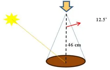
Paper sheets were located in the spectralon height (7 cm) one after another on the ground. Thus the background was changed from red to green and finally to blue. The importance of paying attention to paper heights was because of the scale of our measurements in lab. Afterwards, considering the Field Of View (FOV) of the ASD which is equal to 25˚ in default, the Ground FOV (GFOV) was determined with a circle which has a diameter of 10 centimeters and the measurements’ height was fixed in 46 centimeters respect to the background’s surface. The schematic view of the mentioned experimental set up is presented in Figure 3.

Figure 3: A schematic view of the experimental set up for spectral measurements in the laboratory

In the next step, the fractional abundances of the understudy endmembers changed in various percentages presented in Table 2.

Different fractional abundances were prepared by putting various numbers of sections on the backgrounds. This process is shown in Figure 4.

The International Archives of the Photogrammetry, Remote Sensing and Spatial Information Sciences, Volume XL-1/W5, 2015 International Conference on Sensors & Models in Remote Sensing & Photogrammetry, 23–25 Nov 2015, Kish Island, Iran

(3)

Figure 4: Various abundances were measured using different number of colourful celloluse sections on the background. The FOV region was drawn by using graphical instruments.

3. LINEAR SPECTRAL MIXTURE MODELING

If the total surface area is considered to be divided proportionally according to the fractional abundances of the endmembers, then the reflected radiation will convey the characteristics of the associated media with the same proportions. In this sense, there exists a linear relationship between the fractional abundance of the substances comprising the area being imaged and the spectra in the reflected radiation. Hence, it is called the linear mixing model (LMM) (Cloutis 1996, Chang and Heinz 2000, Meer and Jong 2001, Wim, Janssen et al. 2001, Chang 2003, Clark, Swayze et al. 2003, Keshava 2003, Chang 2007, Bannon 2009, Meer, Werff et al. 2012). When M endmembers exist, each having L distinct spectral bands, and it is expressed as

Equation (1)

where x is the L×1 received pixel spectrum vector, S_{is the}_L× M matrix whose columns are the L×1 endmembers, si,i=1,...,M , a_{is the}_M×1_{fractional abundance vector whose entries are}_ai and w_{is the}_L×1_{additive observation noise vector.}

Assuming that the linear mixing model holds, it is expected that the spectral signatures in calculation and observation being exactly the same. It means that if calculated and observed signatures are considered as y- and x- axes of a scatterplot respectively, then data points will be present on diagonal axis and the linear equation will follow the y=x (See Figure 5).

Figure 5: The expected scatter plot when LMM holds.

4. EXPERIMENTAL RESULTS

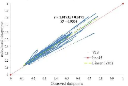
The results of this laboratory experiment indicate that although there was a linear trend line for all data points (various abundances), this line was not coincide with the y=x. Therefore

the assumption of linearity in the mixing model did not hold precisely. Hence, a correction term should be applied in the linear model before any unmixing purpose.

Figure 6, shows the equation of the linear trendline and datapoints dispersion in the scatterplot.

Figure 6: Observed points in the scatter plot, in the 400-800 nm spectral range.

Consequently, a correction term must be applied to the gains and offsets in the linear model (in the 400-800 nm spectral range). This correction term is presented in Equation 2.

Equation (2)

in which, Scorr

is the corrected spectral signature, SLSMA

is the calculated spectra considering linear mixing model.

5. JUSTIFICATION OF THE PROPOSED CORRECTION IN SATELLITE IMAGES

Before drawing any firm conclusion about the proposed correction term, we should prove that our laboratory measurements can simulate the real satellite data. Therefore, we can compare the results with remotely- based images.

First, the measurement height is scaled from around 600 km to 46 cm, and this is the case for the radiation source. Second, the surface roughness of the sheets made of cellulose materials (in millimeter scale), is equivalent to the earth surface topography. The mentioned simulation is illustrated in Figure 7.

Figure 7: A schematic view of the space-borne data acquisition and its simulation with our laboratory measurement from two 3D surfaces

(4)

6. CONCLUSION

The outcome of this laboratory test indicate that the presence of 3D structures in the image cause a deviation from y=x linear equation. Hence, a correction term must be applied to the gains and offsets in the linear model.

Since this study was done in 400-800 nm spectral range, results and the correction terms are proposed only for the same spectral range. Besides, it is expected that the correction terms differ in various spectral ranges; therefore we suggest continuing the work in other spectral ranges as well as other material types.

REFERENCES

Altmann, Y., A. Halimi, N. Dobigeon and J.-Y. Tourneret (2012). "Supervised nonlinear spectral unmixing using a postnonlinear mixing model for hyperspectral imagery." Image Processing, IEEE Transactions on 21(6): 3017-3025.

Bannon, D. (2009). "Hyperspectral imaging: Cubes and slices." Nature Photonics3: 627-629.

Chang, C.-I. (2007). Hyperspectral data exploitation: theory and applications, John Wiley & Sons.

Chang, C. I. (2003). Hyperspectral imaging: Techniques for spectral detection and classification, Wiley publication. Chang, C. I. and D. C. Heinz (2000). "Constrained subpixel terget detection for remotely sensed imagery." IEEE TRANSACTIONS ON GEOSCIENCE AND REMOTE SENSING 38: 1144-1158.

Clark, R. N., G. A. Swayze, K. E. Livo, R. F. Kokaly, S. J. Sutley, J. B. Dalton, R. R. McDougal and C. A. Gent (2003). "Imaging spectroscopy: Earth and planetary remote sensing with the USGS Tetracorder and expert systems." J. Geophys. Res. 5: 1-44.

Cloutis, E. A. (1996). "Review Article Hyperspectral geological remote sensing: evaluation of analytical techniques." International Journal of Remote Sensing 17(12): 2215-2242.

Devices, A. S. (1999). Inc.(ASD) Technical guide, Boulder USA: Analytical Spectral Devices, Inc.

Goodman, J. and S. L. Ustin (2007). "Classification of benthic composition in a coral reef environment using spectral unmixing." Journal of Applied Remote Sensing 1(1): 011501-011501-011517.

Harsanyi, J. C. and C.-I. Chang (1994). "Hyperspectral image classification and dimensionality reduction: an orthogonal subspace projection approach." Geoscience and Remote Sensing, IEEE Transactions on 32(4): 779-785.

Heylen, R., D. Burazerović and P. Scheunders (2011). "Non -linear spectral unmixing by geodesic simplex volume maximization." Selected Topics in Signal Processing, IEEE Journal of 5(3): 534-542.

Keshava, N. (2003). "A survey of spectral unmixing algorithms." Lincoln Laboratory Journal 14(1): 55-78.

Keshava, N. and J. F. Mustard (2002). "Spectral unmixing." Signal Processing Magazine, IEEE 19(1): 44-57.

Meer, F. D. v. d., H. M. A. v. d. Werff, F. J. A. v. Ruitenbeek, C. A. Hecker, W. H. Bakker, M. F. Noomen, M. v. d. Meijde, E. J. M. Carranza, J. B. d. Smeth and T. Woldai (2012). "Multi- and Hyperspectral geologic remote sensing: A review." International Journal of Applied earth observation and geoinformation-ELSEVIER 14: 112-128.

Meer, F. V. and S. M. d. Jong (2001). Imaging spectrometry, Basic principles and prospective applications

Newyork, Boeston, Kluwer academic publishers.

Neville, R., K. Staenz, T. Szeredi, J. Lefebvre and P. Hauff (1999). Automatic endmember extraction from hyperspectral data for mineral exploration. Proc. 21st Can. Symp. Remote Sens.

Rogge, D. M., B. Rivard, J. Zhang and J. Feng (2006). "Iterative spectral unmixing for optimizing per-pixel endmember sets." Geoscience and Remote Sensing, IEEE Transactions on 44(12): 3725-3736.

Wim, H., Bakker, L. F. Janssen, C. Reeves, B. Grote, C. Pohl, M. J. Weir, J. Horn, Prakash. A. and T. Woldai (2001). Principles of Remote Sensing, An introductory textbook. ITC Enscede The Netherlands, ITC EDUCATIONAL TEXTBOOK SERIES