INVESTIGATION OF LATENT TRACES USING INFRARED REFLECTANCE
HYPERSPECTRAL IMAGING
Till Schubert, Susanne Wenzel, Ribana Roscher, Cyrill Stachniss
Department of Photogrammetry, Institute of Geodesy and Geoinformation, University of Bonn, Germany (s7tischu, susanne.wenzel, rroscher)@uni-bonn.de, [email protected]
Commission VII, WG VII/4
KEY WORDS:Hyperspectral Imaging, Forensics, Infrared Spectroscopy, Classification, Random Forest, Markov Random Fields
ABSTRACT:
The detection of traces is a main task of forensics. Hyperspectral imaging is a potential method from which we expect to capture more fluorescence effects than with common forensic light sources. This paper shows that the use of hyperspectral imaging is suited for the analysis of latent traces and extends the classical concept to the conservation of the crime scene for retrospective laboratory analysis. We examine specimen of blood, semen and saliva traces in several dilution steps, prepared on cardboard substrate. As our key result we successfully make latent traces visible up to dilution factor of 1:8000. We can attribute most of the detectability to interference of electromagnetic light with the water content of the traces in the shortwave infrared region of the spectrum. In a classification task we use several dimensionality reduction methods (PCA and LDA) in combination with a Maximum Likelihood classifier, assuming normally distributed data. Further, we use Random Forest as a competitive approach. The classifiers retrieve the exact positions of labelled trace preparation up to highest dilution and determine posterior probabilities. By modelling the classification task with a Markov Random Field we are able to integrate prior information about the spatial relation of neighboured pixel labels.
1. INTRODUCTION
Detecting latent traces is a key field of forensics. Light illumi-nation and screening by goggles form the public image of crime scene investigation. The need for instant examination and clear-ance of the crime clarifies the importclear-ance of efficient and compre-hensive techniques. Chemical contrast enhancement techniques, such as leucocrystal violet treatment and luminol searches, are two of the main methods used to analyse crime scenes. A com-mon contact free method for the task is the use of forensic light sources (FLS), which combines illumination and detection of light by established combinations of forensic lamps and camera filters or goggles, specific for each expected latent trace. We believe that the use of hyperspectral imaging (HSI) (1) allows for analysis of several traces at once, (2) extends the classical concept to the conservation of the crime scene for retrospective laboratory analysis, and (3) leads to a tremendous reduction of time effort. In this paper, we expose biological traces to light of a wide range as well as record its reflectance in many different light colors in infrared (IR) light spectrum (940 to 2543 nm). The goal is to investigate, to what extent, methods from image processing, pattern recognition, and hyperspectral remote sensing are appli-cable in this domain and can be integrated into the investigation of latent traces. This paper gives an overview of the current state of research in forensic spectroscopic applications and presents an approach to analyse forensic traces addressing criminal investi-gators and researchers.
1.1 Task
Guided by the applications in forensics, we investigate two tasks: First, the visualization of latent traces by spectroscopic examina-tion, and second, the automatic detection of latent traces by pixel-wise classification. The former aims at the enhancement of con-trast of latent traces with respect to the background. For that, we select suitable features or extract new features from hyperspec-tral spectra, which are characteristic for each specimen. The lat-ter aims at delat-termining the positions of traces, i.e. a classification
procedure on the task of identification of specimen with unknown trace positioning. We investigate different supervised learning approaches, in order to distinguish trace and background or traces among themselves. All of them result in a posteriori probabilities, which allow to smooth the results by a post-processing step using a Markov Random Field (MRF) to incorporate the dependency of neighbouring pixels.
The work of Edelman (2014) serves as the main reference for de-tection of latent traces using hyperspectral imaging. We adopt the band and ratio method for contrast enhancement and additionally provide the development of spectral indices for FLS similar to Lee and Khoo (2010) and Edelman et al. (2012). For FLS and spectroscopic properties of forensic traces, we refer to Stoilovic (1991) dealing with the absorption behaviour of semen and blood and its light sources for detection.
Our contribution is the proposal of important spectral regions and indices (i.e. combinations of light colors) for the use of forensic light sources and hyperspectral imaging each associated to the responsible biological components, so that classification through common pattern recognition techniques can be applied. Further-more, we provide catalogue wavelengths for direct application in forensic light sources. We evaluate the suitability of hyperspec-tral imaging for crime scene application and provide an outlook for further extensions.
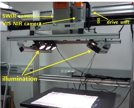
Figure 2: Setting for the image acquisition. Two cameras are located at center top edge of the image facing downwards. The visible near infrared camera did not take part in the experiment.
2. TRACES AND DATABASE
A set of specimen is provided, which comprises the traces blood, semen and saliva. Three cardboard substrates, one for each trace, contain three stains in six dilutions each, thus arranged in three columns and six rows depicting the dilution rates undiluted, 1:2, 1:16, 1:125, 1:1000 and 1:8000. The dilution liquid is water. The visual detectability of the traces is strongly varying, cf. Fig-ure 1. For example, blood is clearly visible in undiluted condition as well as up to dilution rate of 1:125, semen up to 1:16. Saliva is even barely visible in pure condition. To allow for supervised classification, and evaluation of results, we realize ground truth through a coordinate grid, indicated by markers on the border, and depositing traces at the grid points.
For the data acquisition we use a SPECIM shortwave infrared (SWIR) hyperspectral line scanning camera, in the spectral range of940to2543nm, i.e. SWIR light and parts of NIR light. The spectral range is captured within256wavelength bands. The cap-turing setup, cf. Figure 2, therefore requires a one-dimensional movable positioning system (drive unit). For image acquisition, the camera and illumination system are moved with constant ve-locity over the specimen. In advance of the recording, regarding an optimal sensitivity of the camera sensor, we adjust aperture, exposure time and height over the specimen beforehand. The number of pixels, acquired for an image, depends on the res-olution of the line sensor in one direction and on the scan distance in the other, while the former additionally restricts the height of the cameras above the specimen. The SWIR-camera samples 314 pixels arranged in the line sensor. The illumination is provided by six lamps emitting a polychromatic white light of visible and ul-traviolet (UV)-region, as it is comparable to sunlight, which emits the whole spectrum. Using the camera system, we perform image acquisition in emission mode under laboratory conditions, i.e. we illuminate with a fixed excitation light, while recording the emis-sion spectrum over the hyperspectral range. Finally, our database are hyperspectral images showing each specimen separately. For a multiclass application we can, however, handle pixels of differ-ent images jointly, which makes image normalization necessary.
We denoteI¯λthe intensity captured at a certain wave lengthλ. If it is clear from context we skip the index to denote any intensity valueI. As a data pre-processing step we aim at reflectance in-tensity valuesIbeing normalized between minimal and maximal
intensity. In order to achieve this, we put a white reference into the image, next to the specimen during the image scan. The ma-terial, made of barium sulfate, is highly reflective over the whole spectrum providing a 100% reflectance standardI¯ref. After the image acquisition the aperture is closed and the dark response
¯
Idarkis measured.Therefrom, we derive normalized reflectance in-tensity values by
I= I¯−I¯dark ¯
Iref−I¯dark
. (1)
3. VISUALIZATION OF TRACES BY SPECTROSCOPIC EXAMINATION
This section focuses on our first task, the visualization of latent traces. We describe features derived from captured intensities, which we will use to analyse spectroscopic properties of pure and latent traces concerning absorbance and reflectance characteris-tics, in order to make latent traces visible. Using these features, we will investigate, in our experiments, which light colors (i.e. detection wavelengths) cause an enhancement of contrast includ-ing comparison to FLS.
3.1 Spectral Indices
Spectral indices, such as the normalized differenced vegetation index (NDVI), used in remote sensing, are a common device for deriving features from hyperspectral data. In contrast to single wavelength bands, substraction and rationing of images is capa-ble of suppressing background interference and variations in illu-mination (Wagner, 2008; Bao et al., 2009). Ratio images describe a pixelwise difference of intensity values of two wavelengthsλi andλjnormalized by their sum
I(λi,λj)=
Iλi−Iλj Iλi+Iλj
. (2)
A non-normalizing ratio of the formIλi/Iλj and other calcula-tions, such as bracketing an absorption peak by two wavelengths are also reported to eliminate background influence and enhance contrast (Wagner, 2008).
3.2 Fisher’s Ratio
Fisher’s ratio is a measure for the discriminative power of classes. It is based on the assumption that maximal separation is obtained when classes have a large inter-class variability while having a low intra-class variability. The fraction of both is defined as Fisher’s ratio (also F-ratio). Given the vectorsfgxandbgx, con-taining all 1D samples of the respective classes fg and bg, stand-ing for foreground and background, we evaluate their meansfg/bgµ and standard deviationsfg/bgσ, respectively, to obtain Fisher’s ratio by
F fg
x,bg
x
= bgµ
− fgµ2
fgσ2+ bgσ2 , (3) which can be generalized for the multi-class case (Casella, 2008). Please note, that the representation by mean and standard devia-tion assumes Gaussian distributed data. The Fisher’s ratio is the same as Fisher’s criterion, which gets applied in Linear Discrim-inant Analysis.
{(r, c)|y=fg}in vectorfgx
λi = [Iλi](r,c)|y=fg and all other withinbgx
λi = [Iλi](r,c)|y=bg . For each wavelength and each class, we obtain meansfgµ
λi and
bgµ
λi and standard deviations
fgσ
The Ratio image method uses spectral indices of two wave-lengthsλij = [λi, λj], as given in (2), as featuresfgxλij = tively. For each pair of wavelengths and each class we ob-tain meansfgµ
λij and
bgµ
λij and standard deviations
fgσ
xλij and estimate Fisher’s ratio of ratio
images by
The Ratio image method requires two iterations over the spectral dimension. Due to the commutative property if the ratio images, we obtain(n2−n)/2combinations of wavelengths.
In order to identify single bands λi and pairs of wavelength
λij, which maximises the contrast between specimen and back-ground, thus best class separability, we maximise the according Fisher ratios
Identified wavelengths, together with the respective maximal Fisher-ratios, allow exposition of spectroscopically important wavelength bands and indices and comparison of detectability be-tween different cameras and traces.
4. CLASSIFICATION
This section aims at our second task, the automatic detection of latent traces. As we are interested in identifying the positions of the traces on the fabrics, we are dealing with the task of separat-ing foreground and background and the question for each pixel of the image whether it is trace or not, i.e. a classification pro-cedure on the task of identification of traces. We shortly review the methods for supervised classification we use and describe the different procedures we choose for our experiments.
For evaluation we apply different classifiers partially based on methods of dimensionality reductions. As classifiers we consider maximum likelihood (ML) and Random Forest (RF). Principal Component Analysis (PCA) provides dimensionality reduction prior to Linear Discriminant Analysis (LDA), which itself re-duces to one dimension, in the two-class case. All methods are pixel-wise, solely dealing with the spectral feature space. Finally, we smooth the classification results by a MRF, incorporating the spatial arrangement of the pixels in a grid-structure and the evi-dence for each pixel given by the probabilistic output the classi-fier.
Again, we denote feature vectors byx, which may differ for vari-ous contexts, and class labels byy∈ {background, blood, semen, saliva}. We collect feature vectors of all pixels within data matrix Xand their according labels within vectory.
4.1 Dimensionality Reduction
Dimensionality reduction methods are essential for a classifier to extract important features of the data, on which the decision function is based. PCA and LDA present an unsupervised and a supervised method for dimensionality reduction. Due to a num-ber of samples for training, which is lower than the numnum-ber of dimensions, we use PCA to reduce the dimensionality of the fea-ture space. In the supervised approach, we intend to project data to an one-dimensional subspace, in which thresholding serves as classifier. Thus, PCA is optionally performed prior to LDA. In the subspace estimated from LDA we use ML to obtain an opti-mal threshold decision. We fit Gaussian distributions to the data of each class, resulting in the Gaussians’ intersections as class boundaries.
4.2 Random Forest
Random Forest is a classifier combining an ensemble of t = 1. . . T decision trees using majority voting of the most popular decision over all randomly subsampled trees (Breiman, 2001). We obtain a posteriori probabilities for classified samples by learning discrete distributions in the leaf nodes of each tree. Nor-malized categorical histograms, i.e. frequencies of classes in the leafs, build up the discrete probability distributionPt(y|x), which contribute to an average
P(y|x) = 1
over the leaf nodes of all treesT, which the samplexreaches (Chawla and Cieslak, 2006).
4.3 Markov Random Field
To combine prior knowledge about the spatial relations between neighboured pixels with our evidence about each pixels class, given by the probabilistic output of the classifier, we model our classification task as a MRF, which is given by
P(y|X) = 1/Z·exp−P
ilogP(yi|xi)−w·P(i,m)∈Niδ(yi, ym)
.
(9) The first, unary term is defined as the negative logarithm of the posteriorsP(yi|xi)obtained by the classifier. Since we assume the final labelling of the pixels to be smooth within the image, we introduce this prior knowledge by means of a Potts model in the second, binary term. The term describes the interaction potential over a 2D lattice penalizing every dissimilar pair of labels and therefore heterogeneous regions utilizing the Kronecker function δ. The set of spatial neighbours is denoted byNi. The variable
wis the weight between both terms and the normalization con-stant is given byZ. We use max-product to solve for the best labellingy˜= argmaxyP(y|X), while weightwis empirically
determined, see (Bishop, 2006, Chapter 8.4.5).
5. EXPERIMENTAL RESULTS
Training and test data were collected by picking pixels within a circle of fixed radius, at the grid positions, specified by markers at the border of the specimen, and samples for background from regions in between. We take two third as training data leaving one third as test data. Please note, that capturing of foreground pixel was done automatically, thus not as accurate as pixel-wise labelling. To avoid false data for training, we choose the radius of the circles for region of interest small, thus we expect real ground truth to be larger as we labelled.
5.1 Visualization of Traces by Spectroscopic Examination
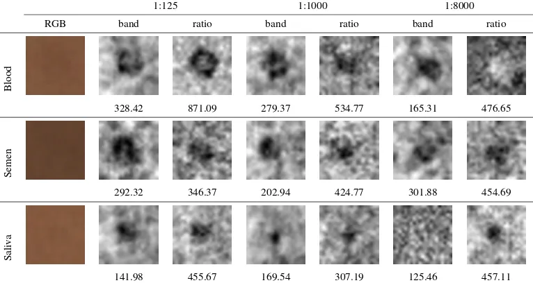
Figure 3 contains visualizations of the regions around the stains. We display the images at bandIλiand ratioI(λi,λj), which were
identified as most discriminative by Fisher’s ratioFλiandFλij,
respectively. We perform distinction with the respective dilu-tion of each stain against background and indicate the resulting maximal F-ratio (i.e. the measure for the detectability) under-neath the images. Band and ratio image show the same stain for each dilution. We observe that band and ratio images provide enhanced differences between trace and background. Thus, we make traces visible when RGB-view does not provide recogni-tion. However, we realize that ratio images provide a better fea-ture definition than single wavelength bands. We can clearly see that the value of Fisher’s ratio is representative for the detectabil-ity in the grayscale images.
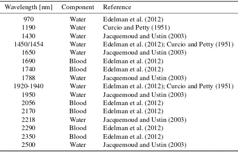
Table 1 lists up all wavelengths and Fisher’s ratios allocated for dilutions, while Table 2 contains a list of spectral peaks, in range of SWIR, of several trace components as reported in the literature. Bold values in Table 1 indicate correspondences to trace-specific absorption peaks and italic notation signifies accordance to water peaks. The dominance of water interference is clearly given. Nearly each band and ratio contains at least one wavelength at an established water peak. Consequently, we can attribute most of the detectability of traces to the amount of water in the traces. Even blood features more accordances with water peaks than with hemoglobin influence.
5.2 Binary Classification
We show segmentation images as binary (black-white) images for binary classification in Figure 4. We realize that the SWIR-images provide good classification and reconstruction of the stains. All traces are successfully classified up to highest dilu-tion. Visually, the best classifier is ML based on PCA and LDA. The Random Forest, however, exhibits connected misclassified regions instead of noise.
The postprocessing step successfully achieves to reduce noisy
Table 1: Wavelengths with maximal Fisher’s ratios calculated for different methods (band, ratio) and different dilution rates of blood in SWIR-data, including accordances to established ab-sorption peaks as given in Table 2. Bold values indicate corre-spondences to trace-specific absorption peaks. Italic notation sig-nifies accordance to water peaks.
Dilution undiluted 1:2 1:16 1:125 1:1000 1:8000 all
Band 1598 1573 1937 1906 1900 1900 1906
Ratio 1598 1573 1585 1944 1944 1919 1937 Blood 1831 1862 1862 2188 2107 2169 2138
Band 2169 2232 1994 1894 1894 1900 1906
Ratio 1428 1453 1956 1950 1950 1497 1956 Semen 1994 1994 2063 2113 2175 1900 2063
Band 1956 1950 1937 1925 1937 959 1937
Ratio 1440 1440 1503 1535 1535 1092 1535
Sali
v
a
1956 1981 1956 1925 1956 1956 1937
Table 2: List of spectral peaks, in range of SWIR, of several trace components as reported in the literature. The component blood comprises hemoglobin, albumin, and globulin.
Wavelength [nm] Component Reference
970 Water Edelman et al. (2012) 1190 Water Curcio and Petty (1951) 1430 Water Jacquemoud and Ustin (2003)
1450/1454 Water Edelman et al. (2012); Curcio and Petty (1951) 1650 Water Jacquemoud and Ustin (2003)
1690 Blood Edelman et al. (2012) 1740 Blood Edelman et al. (2012) 1788 Water Jacquemoud and Ustin (2003)
1920-1940 Water Edelman et al. (2012); Curcio and Petty (1951) 1950 Water Jacquemoud and Ustin (2003)
2056 Blood Edelman et al. (2012) 2170 Blood Edelman et al. (2012) 2218 Water Jacquemoud and Ustin (2003) 2290 Blood Edelman et al. (2012) 2350 Blood Edelman et al. (2012) 2500 Water Jacquemoud and Ustin (2003)
classification. Nonetheless, the approach fails on the connected misclassified regions of Random Forest. In case of ML based on PCA and LDA, we can entirely retrieve the ground truth la-belling mask. All images show that the identification of traces is accomplished clearly beyond visual detectability.
5.3 Multiclass Classification
Next, we investigate the multiclass performances of the classi-fiers. We show results for the multiclass approach in Figures 5 and 6. Next to the segmentation images we display the RGB-image (true-color). Although each specimen is captured in an own image, we can handle them jointly, due to performed image normalization.
We observe that the RF outperforms the ML approach, cf. Figure 5. Blood and saliva are classified correctly up to the highest dilution, semen can only be retrieved up to dilution 1:2. It is noticeable that a fringe around a stain of blood is classified as semen. The ML classifier assumes nearly all traces as blood and exhibits higher noise in background regions. For both classifiers, background is mostly confused with saliva. Traces tend to attain blood labels if classified falsely.
A qualitative evaluation, in terms of confusion matrices, provides the same result, cf. Table 3. Using Random Forest, Table 3 left, 93% of background, 66% of blood, 35% of semen and 75% of saliva pixels are classified correctly. The overall accuracy amounts to76.2%. Semen is assigned to other classes in large quantities. The accuracies of the ML, Table 3 right, approach completely decline. Overall accuracy adds up to65.5%. Classi-fication of semen is particularly vague because48%and29%are misassigned to blood and saliva leaving21%correct allocations. Nonetheless, confusion with background is partially lower than for the RF classifier.
Table 3: Confusion matrix with classwise accuracies for multi-class multi-classification.
Prediction
RF ML / LDA / PCA backg. blood semen saliva backg. blood semen saliva
backg. 0.934 0.009 0.009 0.049 0.881 0.000 0.000 0.119 blood 0.173 0.660 0.013 0.153 0.000 0.640 0.233 0.127
T
ruth
1:125 1:1000 1:8000
RGB band ratio band ratio band ratio
Blood
328.42 871.09 279.37 534.77 165.31 476.65
Semen
292.32 346.37 202.94 424.77 301.88 454.69
Sali
v
a
141.98 455.67 169.54 307.19 125.46 457.11
Figure 3: Best band and ratio imagesIλiand ratioI(λi,λj), identified by maximal Fisher’s ratiosFλiandFλi, respectively, given by
numbers under each image. According bandsλiand wavelengths pairsλi,jare given in Table 1.
Blood
Semen
Saliva
(a) (b) (c) (d) (e) (f)
Figure 4: Results for binary classification. Traces on each speci-men are provided, such that the fraction of dilution increases from top to bottom. Columns: a) RGB, b) ground truth, c) RF, d) PCA/LDA and ML, e) RF followed by MRF, f) PCA/LDA and ML followed by MRF.
(a) Blood (b) Semen (c) Saliva
Figure 5: Results of multiclass classification. Columns for each specimen:Left- RGB.Middle- RF.Right- PCA and LDA fol-lowed by ML. Meaning of colours given in the colour bar. (Best viewed in colour.)
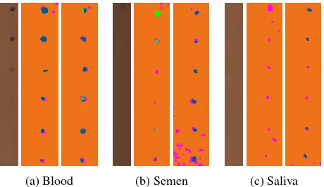
For the mutliclass approach, MRF postprocessing does not yield as accurate results as the binary case, cf. Figure 6. Despite reduc-tion of noise, we now obtain stains entirely occupied by a false class. Thus, we predominantly classify the water content of the traces instead of the individual trace itself. The traces seem to intersect due to dilution. We present a quantitative evaluation in terms of confusion matrices in Table 4. By postprocessing we can increase the classwise accuracies, mostly for blood. Confusion of some traces is reduced to zero as a consequence of reduced noisy misclassification. We can see that predominantly the strongest class receives more classified samples. Thus, in case of PCA, LDA, and ML the wrong classes get eliminated.
Table 4: Confusion matrix with classwise accuracies for multi-class multi-classification postprocessed by MRF.
Prediction
RF ML / LDA / PCA backg. blood semen saliva backg. blood semen saliva
backg. 1.000 0.000 0.000 0.000 1.000 0.000 0.000 0.000 blood 0.167 0.773 0.000 0.060 0.007 0.820 0.127 0.046
T
ruth
(a) Blood (b) Semen (c) Saliva Figure 6: Results of multiclass classification postprocessed by MRF. Columns for each specimen: Left- RGB. Middle- RF. Right- PCA and LDA followed by ML. Colours as given in Fig-ure 5. (Best viewed in colour.)
6. CONCLUSIONS
Latent traces have been successfully made visible exploiting hy-perspectral data. The detectability can be significantly improved towards single wavelength images by the calculations of bands. A spectroscopic examination shows that detection of latent traces is predominantly water based. However, not the same regions of interference with water are relevant for the single traces. The SWIR-region accounts for excellent visibility of traces in band and ratio images up to the highest dilution (1:8000). We provide various options of normalized differenced indices (ratio images) and band images.
Besides visual detectability, a classification approach has shown to what extent traces on fabrics can be labelled as such. We have successfully retrieved the positions in a classification task in SWIR-data up to maximal dilution (1:8000). Various classi-fiers have presented different forces and weaknesses towards the data. Random Forest and LDA in connection with a PCA pro-vide the best classifiers. The evaluation from segmentation im-ages favours LDA with PCA due to less connected regions and few widespread misclassified pixels. This is a sign that Gaussian distribution are appropriate for the data. For the multiclass case Random Forest yields best results. In an additional modelling of the classification task by a MRF we achieve smoother segmen-tation images by reduction of noisy classification, which exactly recovers the labelled regions.
Despite our encouraging results, there is further space for im-provements. In order to achieve better results and an applica-tion to arbitrary images and specimen an increased control over background influences (i.e. inducing trace-specific interactions) is recommended. Supervision by targeted initiation of only trace-specific interference by appropriate illumination and variation over single bandpass light colors (i.e. excitation measurement mode) has to be considered. A possible extensions is the assimi-lation of excitation-emission maps (EEM) providing a modelling of the relation between excitation and emission as well as scatter corrections.
This work has revealed the IR-region principal for biological traces. For the SWIR-camera higher resolutions are essential. Referring to Edelman et al. (2015) area scanning cameras with tunable filters are preferable and achieve a proper spatial resolu-tion as well as easier reposiresolu-tioning at the crime scene. Next to that, they allow simpler live view (in situ) applications. Single band images and ratio images can be directly visualized on an external screen. Line-scanning cameras require on-the-fly image normalization for this task. As a conclusion, the investigation of the applicability of hyperspectral imaging for the detection of latent traces has revealed to have reasonable potential.
ACKNOWLEDGEMENTS
We thank the State Office of Criminal Investigations of North Rhine-Westfalia in D¨usseldorf who provided all specimen. We also thank Anne-Katrin Mahlein from department of Plant Dis-eases and Plant Protection of the Institute of Crop Science and Resource Conservation (INRES) of the University of Bonn who supported the image acquisition.
References
Bao, Y., Gao, W. and Gao, Z., 2009. Estimation of winter wheat biomass based on remote sensing data at various spatial and spectral resolu-tions. Frontiers of Earth Science in China 3(1), pp. 118–128.
Bishop, C. M., 2006. Pattern Recognition and Machine Learning (Infor-mation Science and Statistics). Springer.
Breiman, L., 2001. Random Forests. Machine learning 45(1), pp. 5–32.
Casella, G., 2008. Statistical design. 1 edn, Springer Science & Business Media.
Chawla, N. V. and Cieslak, D. A., 2006. Evaluating probability estimates from decision trees. American Association for Artificial Intelligence.
Curcio, J. A. and Petty, C. C., 1951. The near infrared absorption spec-trum of liquid water. Journal of the Optical Society of America 41(5), pp. 302–302.
Edelman, G. J., 2014. Spectral analysis of blood stains at the crime scene. PhD thesis, Faculty of Medicine, University of Amsterdam.
Edelman, G. J., Manti, V., van Ruth, S. M., van Leeuwen, T. and Aalders, M., 2012. Identification and age estimation of blood stains on colored backgrounds by near infrared spectroscopy. Forensic Sci Int 220(1-3), pp. 239–244.
Edelman, G. J., van Leeuwen, T. G. and Aalders, M. C., 2015. Visu-alization of latent blood stains using visible reflectance hyperspectral imaging and chemometrics. J Forensic Sci 60, pp. 188–192.
Jacquemoud, S. and Ustin, S. L., 2003. Application of radiative transfer models to moisture content estimation and burned land mapping. In: 4th International Workshop on Remote Sensing and GIS Applications to Forest Fire Management, pp. 3–12.
Lee, W. C. and Khoo, B. E., 2010. Forensic light sources for detection of biological evidences in crime scene investigation: a review. Malaysian J. Forensic Sci 1, pp. 17–28.
Stoilovic, M., 1991. Detection of semen and blood stains using polilight as a light source. Forensic Sci Int 51(2), pp. 289–296.