NDVI FROM LANDSAT 8 VEGETATION INDICES TO STUDY MOVEMENT
DYNAMICS OF
CAPRA IBEX
IN MOUNTAIN AREAS
Francesco Pirottia* Maria A. Parragab, Enrico Stuarob, Marco Dubbinib, Andrea Masieroa, Maurizio Ramanzinb
a CIRGEO Interdepartmental Research Center of Geomatics, Università degli Studi di Padova, viale dell’Università 16, 35020 Legnaro (PD) Italy – (francesco.pirotti, andrea.masiero)@unipd.it
b DAFNAE Department of Agronomy Food Natural Resources Animal and Environment, Università degli Studi di Padova, viale dell’Università 16, 35020 Legnaro (PD) Italy – (enrico.stuaro, maria.parraga,
maurizio.ramanzin)@unipd.it
Commission VII
KEY WORDS: Capra ibex, Landsat 8, Vegetation indices, Ethology modelling, Pseudo invariant features.
ABSTRACT:
In this study we analyse the correlation between the spatial positions of Capra ibex (mountain goat) on an hourly basis and the information obtained from vegetation indices extracted from Landsat 8 datasets. Eight individuals were tagged with a collar with a GNSS receiver and their position was recorded every hour since the beginning of 2013 till 2014 (still ongoing); a total of 16 Landsat 8 cloud-free datasets overlapped that area during that time period. All images were brought to a reference radiometric level and NDVI was calculated. To assess behaviour of animal movement, NDVI values were extracted at each position (i.e. every hour). A daily “area of influence” was calculated by spatially creating a convex hull perimeter around the 24 points relative to each day, and then applying a 120 m buffer (figure 4). In each buffer a set of 24 points was randomly chosen and NDVI values again extracted. Statistical analysis and significance testing supported the hypothesis of the pseudo-random NDVI values to be have, in average, lower values than the real NDVI values, with a p-value of 0.129 for not paired t-test and p-value of <0.001 for pairwise t-test. This is still a first study which will go more in depth in near future by testing models to see if the animal movements in different periods of the year follow in some way the phenological stage of vegetation. Different aspects have to be accounted for, such as the behaviour of animals when not feeding (e.g. resting) and the statistical significance of daily distributions, which might be improved by analysing broader gaps of time.
1. INTRODUCTION
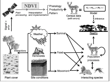
The importance of NDVI comes from the fact that it gives information about a primary production (vegetation) over time. (Pettorelli et al., 2011) have studied such interaction (figure 1) and found significant results related to biological dynamics.
Figure 1. Schematic representation of interaction between vegetation and animals, and how NDVI can be useful (Pettorelli et al., 2011).
NDVI allows to study the species related to this primary production and their behaviour with its changes and can also help the wildlife distribution models (Suárez-Seoane et al., 2004). It is possible to find a lot of information in literature about the correlation of NDVI (as a proxy of vegetation growth) and movement of large herbivores, that is strongly related to the access to better forage (Fryxell and Sinclair, 1988). One example is the study about the interaction between climatic variability (measured by the North Atlantic oscillation ‘NAO’), vegetation phenology and red deer body mass and movement in Norway (Pettorelli et al., 2005a). Results in this investigation show that earlier spring season can cause a faster growth of vegetation that leads to an increase in the body mass and earlier migrations of the animals. Other examples in literature that underline the benefits of NDVI in wildlife studies can be enumerated wth the following investigations:
- Estimation of vegetation growth by NDVI its relation between migration of Connochaetes taurinus in the Serengeti (Boone et al., 2006).
- Correlation between wet-season home-range of elephants and seasonal vegetation productivity in southern Africa (young et al., 2009) or between elephant diet and NDVI variation in Kenya (Wittemyer et al., 2009).
- NDVI can be a good predictor to assess the body mass of roe deer and reindeer in France and Norway (Pettorelli et al., 2006, 2005b).
Another study that is important to discuss is that one done on African buffalo where the correlation between quality of food (using NDVI) and occurrence/synchrony of birth was assessed, then relative relationship between NDVI and presence of nitrogen, that is an important protein surrogate, was investigated with data from field surveys (Ryan et al., 2007) (Figure 2). This underline how NDVI can be a good proxy for estimating vegetation quality for herbivores.
Figure 2. NDVI in grey and monthly births of animal (Ryan et al., 2007)
The story of NDVI is closely correlated to the start of the Landsat program. The launch of the Landsat 1 was in the 1972 and it was integrated with multispectral scanner that allowed to investigate also into the spring vegetation green-up and the subsequent summer and fall dry-down. To overcame the problem of the differences in solar zenith angle cross, Donald Deering, Robert Haas and John Schell developed the ratio of the difference of the red and infrared radiances over their sum as a means to adjust or normalize the effects of the solar zenith angle in the 1973. The normalized difference vegetation index is one of the most useful and used index to quickly identify vegetated areas with the use of multispectral remote sensing data. The NDVI was applied over time in many different aspects:
- Vegetation dynamics/Phenology over time (Wellens, 1997). - Biomass production (Anderson et al., 1993).
- Grazing impacts/Grazing management (Hunt and Miyake, 2006).
- Change detection (Minor et al., 1999)
- Vegetation/Land cover classification (Geerken et al., 2005). - Soil moisture estimation (Wang et al., 2004).
- Wildlife management (Pettorelli et al., 2011)
In the presented investigation our objective was to analyse the distribution of NDVI values in terms of recorded animal position over time. We wanted to assess if any trend is present which shows that either the whole population which is monitored, or any particular individual, have a preference over the choice of the area where it is found at time of recording, and if any trends are present.
2. STUDY AREA AND MATERIALS
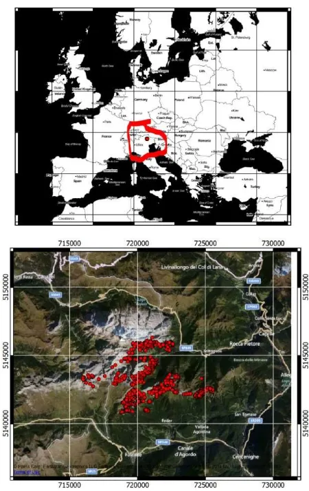
The study area is located in the north-east part of Italy (Figure 3). It is an Alpine region, with steep slopes and a range of heights above sea level between 1700 and 3000 m a.s.l. In this area there is the presence of Capra ibex as local fauna. Eight individuals (all females) were tagged with a GPS collar which transmits information of position and acceleration every hour. This allows to monitor eventual deaths of the animal, since it will have the same position over time and no accelerometric information.
The Landsat 8 was launched 11th February 2013 an started to acquire images the 18th of March 2013 (Belward and Skøien, 2014). This sensor provides 16-bit images at 30 m resolution for multispectral bands (10 for panchromatic and 100 for thermal). With respect to Landsat 7, it has an extra band at the low part of
the visible spectrum, therefore the red and infrared bands are respectively the 4th and 5th band instead of the 3rd and 4th like in the Landsat 7 (NASA, 2013).
Figure 3. Different views of the study area; top – regional view and bottom – close-up of the region with the red points representing the positions of the female Capra ibex.
The data received from Landsat 8 are processed using parameters consistent with all standard Landsat data products (table 1) and are available for download at no charge and with no user restrictions from EarthExplorer or the LandsatLook Viewer at http://landsatlook.usgs.gov. (NASA, 2013)
3. METHOD
We analyse the correlation between the spatial positions of Capra ibex (mountain goat) on an hourly basis and the information obtained from vegetation indices extracted from Landsat 8 datasets. Eight individuals were tagged with a GPS collar and their position was recorded every hour since the beginning of 2013 to 2014 for a total of 16 time-stamps corresponding to Landsat 8 datasets which had matching dates. Table 1 shows the number of records from the GPS collar which every hour sends information to the database. The utc_date shows the date of the Landsat 8 image. Where there are 24 readings it means that every hour of the day the positioning information was acquired from the collar during the whole day. The International Archives of the Photogrammetry, Remote Sensing and Spatial Information Sciences, Volume XL-7, 2014
Lower numbers indicate malfunctions or cloud cover which
88320 88360 88390 8840 88400 88410 8842 88420
13/04/2013 22 23 24 0 24 24 0 24
Table 1. Contingency table of number of records per animal for each Landsat 8 image.
88320 88360 88390 8840 88400 88410 8842 88420 TOTAL
00 6 8 7 6 6 7 7 7 54
Table 2. Contingency table with number of records per animal per hour of day.
88320 88360 88390 8840 88400 88410 8842 88420 TOTAL
3 0 0 0 46 0 0 45 0 91
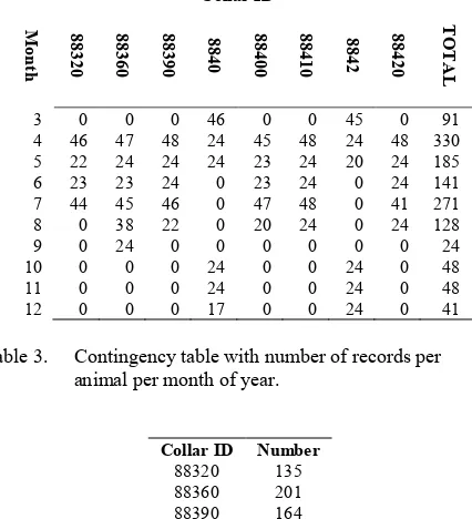
Table 3. Contingency table with number of records per animal per month of year.
Table 4. Summary table of number of records per each monitored animal.
IR and R are respectively the infrared and red band (5th and 4th band respectively), n is the position of the animal.
We applied a normalization procedure using Landsat 8 radiance rescaling factors provided in the metadata file to provide top of atmosphere values (TOA):
L cal L
L
M Q
A
(2)where:
L = TOA spectral radiance (Watts (m-2 srad-1 m-1) ML = Band-specific multiplicative rescaling factor from the metadata for each band number)
AL = Band-specific additive rescaling factor from the metadata for each band number
Qcal = Quantized and calibrated standard product pixel values (DN)
We removed points which were under cloud coverage which leads to misinterpretation of the NDVI value. Pseudo invariant features (PIFs) method (Du et al., 2002) was used on the TOA values to check that the areas that we expect to have invariant reflectance for each band is actually so. All images were The International Archives of the Photogrammetry, Remote Sensing and Spatial Information Sciences, Volume XL-7, 2014
therefore brought to a reference radiometric level and NDVI was calculated.
Figure 4. Daily are of influence plotted over NDVI color map obtained from Landsat 8 satellite
To compare our distribution of NDVI values with a control, we created a random stratified sampling over the daily “area of influence” (AoI) (figure 4). This area was calculated by spatially creating a convex hull perimeter around the 24 points relative to each day, and then applying a 120 m buffer (figure 4). The sampling was stratified according to such areas. In each area a set of 24 points was randomly chosen and NDVI values again extracted with the same process. This can be defined as a pseudo-random sampling, as the randomness is applied to the distance and the direction of the new point, which cannot be the same as the original position. Another term of comparison was the distribution of NDVI values in the AoI, extracting mean and standard deviation from each area, and then using this information for statistical comparison.
4. RESULTS AND DISCUSSION
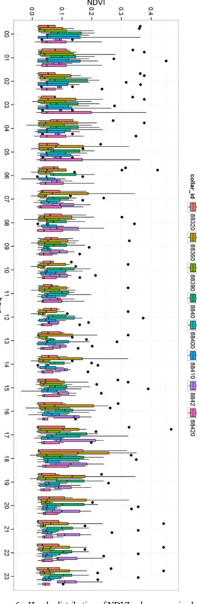
A first look at overall distribution of NDVI as a function of month of the year, and time of day in figure 5 and figure 6 respectively, allows a visual interpretation of any immediate trends that might be evident. We must keep in mind that this are still initial results and that monitoring and data recording are still going on. This dataset requires assessing the different sources of variability, which have to be considered when trying to model relationships between position, time and NDVI values. First of all animal behaviour cannot be considered homogenous, but a subjective aspect related to ethology of the specific species. It cannot be expected that all animals behave in the same way regarding their position in space during time of day and time of year. The variability of the land surface itself is a factor along with the behaviour of Capra ibex, as feeding happens in mountainous areas and it might be the case that a rocky slope hides feeding spots which are not large enough to be recorded by an NDVI value in a 30 m pixel. Another aspect to be mentioned is that we do have a certain number of records (see table 1-3), and it might seem that the numerosity of the sample is enough, but it must be kept in mind that it includes position during night time, were feeding does not take place. Also the seasonal variation in habits of the animal is a factor which must be considered with experts on the field. The ideal procedure would be to relate time of day and day of year to NDVI removing ranges of data to keep only significant sets – e.g. if it is a known fact that animals do not feed during the night, then we might decide to remove data which belongs to
night hours, depending on the season. This would simply be considered a method to limit variability which is not due to the phenomenon under analysis.
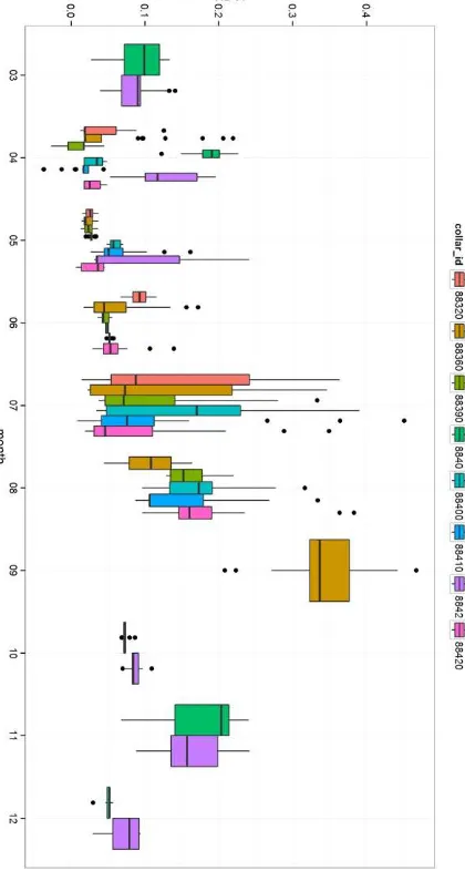
Figure 5. Monthly distribution of NDVI values per animal.
An analysis over figure 5 and figure 6 does give us some input for further analysis. Figure 5 shows that the summer months have data that are more complete, i.e. have a higher number of animal positions, than the winter months. Therefore there is not enough information to infer relationship between season and NDVI at this stage; table 3 confirms this.
4.1 Is the data normally distributed?
To test for normality the Shapiro-Wilk test was applied to the data, and the resulting p-value showed that the data are not distributed normally. A successive analysis using a QQ-plot against a randomly generated normal distribution supported this conclusion. Therefore we cannot consider our data as normal. Nevertheless, because our sample size is quite large, we can proceed to compare distribution and define significant differences using Student t-test and a Wilcoxon signed-rank test. Nevertheless we must keep in mind that is we subset the data to analyse grouped differences, then the non-normal distribution must be considered is the number of samples is less than fifty (Rice, 1995).
Figure 6. Hourly distribution of NDVI values per animal.
4.2 Student t-test
A first test, Student t-test, was applied to the whole dataset to see if the random positions extracted nearby the real positions do give us a significantly different NDVI value.
2 2
a b
a b
a b
x
x
t
s
s
n
n
(3)
where:
a and b are the real and pseudo-random distribution respectively, s is the standard deviation and n the numerosity of the sample (in our case it n = 1307). We choose to apply a one-tailed test to define if the mean of the pseudo-random NDVI values is significantly less than the mean of the real distribution. The result for a difference of means of -0.0037, t = -1.1309 p-value = 0.1291, whereas the p-p-value of a paired t-test was of <0.001. This allows us to say that the difference of means of the two distributions, in the sense that the real NDVI is greater than the pseudo-random ones, are very weakly different, unless we account for paired criteria, were this difference becomes very significant. In this case study the latter can be supported because there is a one-to-one relationship between points, as each “pseudorandom” point was taken from a real point, and the sampling mechanism was applied to distance and direction from the real point, therefore each real point is matched on a one to one basis to a pseudo-random point.
4.3 Wilcoxon signed-rank test
Another test was applied to the whole dataset to see if the random positions extracted nearby the real positions gave us a significantly different NDVI value.
2 1
1
sgn(
) R
N
i i i
i
W
x
x
(5)where:
W is the result of the test, N is the number of ranked pairsr, x2 and x1 are the values of the ith rank pair of values, where i = 1,…,N and Ri is the notation of the ith rank.
The result of the classical Wilcoxon test gave us a p-value of 0.0766, which means a 7.66% probability that the difference in means is due to casuality, and therefore we cannot refute the null hypothesis (H0) at 95% confidence. H0, e.g. the two distributions have the same mean value. Further application of this test applying the continuity correction gave us a p-value 0.00087, which leads to quite different conclusions. Like the Student t test the pair-wise comparison leads to think that we can refute the null hypothesis and that the means are significantly different even at 99.9% confidence level.
These initial results over the full dataset are comforting, because we have, as was mentioned before, many sources of variation, as positions might include resting spots or other relations not related to feeding habits. It is advisable to subset the data, as we suggested, trying to remove unrelated information. This will be the objective for future analysis.
4.4 Monthly differences
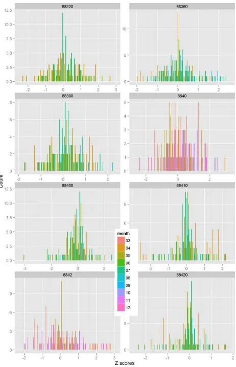
We used a z-score test to extract which differences between real and pseudo-random NDVI are significant using a confidence level of 99%. In figure 7 we plot al the z-scores for each animal, coloured by month to visually assess if there are any significant trends between the time of the year and the difference between the two distributions. The z-score is related to the distribution of the NDVI in the day (~24 records).
Z-score above 2.58 will hold true for a confidence interval of 99% whereas if we drop to 95% confidence interval, the z-score threshold is 1.96. From figure 3 we can see that several cases (days) the difference is significant and we can believe that the behaviour of the animal led to choosing a certain spot instead of the neighbouring areas for a reason. This would lead to discussion on ecological and behavioural trends which are out of scope for this paper.
Statistical analysis was also carried out comparing distributions of NDVI, one for the real positions of the animals, and against the random sampling of points, and for the total NDVI values of the area of influence (AoI). Because we have two distributions in the first case, we applied a z-test over all un-aggregated data to find if there we can expect the real NDVI values were in average higher than the pseudo-random ones. Initial results are reported in figure 5.
Figure 7. Z-scores of differences between real and pseudo-random NDVI.
5. CONCLUSIONS
We tested data of Capra ibex positions over 16 Landsat 8 images using NDVI values. We tested against two controls: (i) the statistical representation of NDVI values of the whole effective area of each animal per day (AoI – area of influence), and (ii) a semi-random distribution acquired by “jittering” the animal position from the original value anywhere else between a radius of 2 to 4 pixels at a random direction away from the original point. Results show that in some cases the differences are significant and represent an interesting source for further study.
In the near future we will go more in depth by testing models to see if the animal movements in different periods of the year follow in some way the phenological stage of vegetation. Different aspects have to be accounted for, such as the behaviour of animals when not feeding (e.g. resting) and the statistical significance of daily distributions, which might be improved by analysing broader gaps of time.
REFERENCES
Anderson, G.., Hanson, J.., Haas, R.., 1993. Evaluating landsat thematic mapper derived vegetation indices for estimating above-ground biomass on semiarid rangelands. Remote Sensing of Environment,. doi:10.1016/0034-4257(93)90040-5
Belward, A.S., Skøien, J.O., 2014. Who launched what, when and why; trends in global land-cover observation capacity from civilian earth observation satellites. ISPRS Journal of Photogrammetry and Remote Sensing,. doi:10.1016/j.isprsjprs.2014.03.009
Boone, R.B., Thirgood, S.J., Hopcraft, J.G.C., 2006. Serengeti wildebeest migratory patterns modeled from rainfall and new vegetation growth. Ecology, 87, 1987–1994.
doi:10.1890/0012-9658(2006)87[1987:SWMPMF]2.0.CO;2
Du, Y., Teillet, P.M., Cihlar, J., 2002. Radiometric
normalization of multitemporal high-resolution satellite images with quality control for land cover change detection. Remote Sensing of Environment, 82, 123–134. doi:10.1016/S0034-4257(02)00029-9
Fryxell, J.M., Sinclair, A.R., 1988. Causes and consequences of migration by large herbivores. Trends in ecology &
evolution (Personal edition), 3, 237–241.
doi:10.1016/0169-5347(88)90166-8
Geerken, R., Batikha, N., Celis, D., DePauw, E., 2005.
Differentiation of rangeland vegetation and assessment of its status: field investigations and MODIS and SPOT VEGETATION data analyses. International Journal of Remote Sensing,. doi:10.1080/01431160500213425 Hunt, E.R., Miyake, B.A., 2006. Comparison of Stocking Rates
From Remote Sensing and Geospatial Data. Rangeland Ecology & Management,. doi:10.2111/04-177R.1 Minor, T.B., Lancaster, J., Wade, T.G., Wickham, J.D.,
Whitford, W., Jones, K.B., 1999. Evaluating change in rangeland condition using multitemporal AVHRR data and geographic information system analysis.
Environmental Monitoring and Assessment, 59, 211– 223. doi:10.1023/A:1006126622200
NASA, 2013. Landsat 8 Fact Sheet 2013–3060 3–6.
Pettorelli, N., Gaillard, J.M., Mysterud, A., Duncan, P., Stenseth, N.C., Delorme, D., Van Laere, G., Toïgo, C., Klein, F., 2006. Using a proxy of plant productivity (NDVI) to find key periods for animal performance: The case of roe deer. Oikos, 112, 565–572.
doi:10.1111/j.0030-1299.2006.14447.x
Pettorelli, N., Mysterud, A., Yoccoz, N.G., Langvatn, R., Stenseth, N.C., 2005a. Importance of climatological downscaling and plant phenology for red deer in heterogeneous landscapes. Proceedings. Biological
sciences / The Royal Society, 272, 2357–2364.
doi:10.1098/rspb.2005.3218
Pettorelli, N., Ryan, S., Mueller, T., Bunnefeld, N., Jedrzejewska, B., Lima, M., Kausrud, K., 2011. The Normalized Difference Vegetation Index (NDVI): unforeseen successes in animal ecology. Climate Research,. doi:10.3354/cr00936
Pettorelli, N., Weladji, R.B., Holand, O., Mysterud, A., Breie, H., Stenseth, N.C., 2005b. The relative role of winter and spring conditions: linking climate and landscape-scale plant phenology to alpine reindeer body mass. Biology
letters, 1, 24–26. doi:10.1098/rsbl.2004.0262
Rice, J. a, 1995. Mathematical Statistics and Data Analysis, Higher Education. doi:10.2307/3619963
Ryan, S.J., Knechtel, C.U., Getz, W.M., 2007. Ecological cues, gestation length, and birth timing in African buffalo (Syncerus caffer). Behavioral Ecology, 18, 635–644. doi:10.1093/beheco/arm028
Suárez-Seoane, S., Osborne, P.E., Rosema, A., 2004. Can climate data from METEOSAT improve wildlife distribution models? Ecography, 27, 629–636. doi:10.1111/j.0906-7590.2004.03939.x
Wang, C., Qi, J., Moran, S., Marsett, R., 2004. Soil moisture estimation in a semiarid rangeland using ERS-2 and TM imagery. Remote Sensing of Environment, 90, 178–189. doi:10.1016/j.rse.2003.12.001
Wellens, J., 1997. Rangeland vegetation dynamics and moisture availability in tunisia: an investigation using satellite and meteorological data. Journal of Biogeography,.
doi:10.1046/j.1365-2699.1997.00159.x
Wittemyer, G., Cerling, T.E., Douglas-Hamilton, I., 2009. Establishing chronologies from isotopic profiles in serially collected animal tissues: An example using tail hairs from African elephants. Chemical Geology, 267, 3– 11. doi:10.1016/j.chemgeo.2008.08.010