ENHANCED MODELING OF REMOTELY SENSED ANNUAL LAND SURFACE
TEMPERATURE CYCLE
Zhaoxu Zou a, Wenfeng Zhan a, b, *, Lu Jiang a
a
Jiangsu Provincial Key Laboratory of Geographic Information Science and Technology, International Institute for Earth System Science, Nanjing University, Nanjing, Jiangsu 210046, China - [email protected], [email protected]
b Jiangsu Center for Collaborative Innovation in Geographical Information Resource Development and Application, Nanjing 210023,
China - [email protected]
KEY WORDS: Thermal remote sensing, Land surface temperature, Enhanced, Modelling, Annual temperature cycle
ABSTRACT:
Satellite thermal remote sensing provides access to acquire large-scale Land surface temperature (LST) data, but also generates missing and abnormal values resulting from non-clear-sky conditions. Given this limitation, Annual Temperature Cycle (ATC) model was employed to reconstruct the continuous daily LST data over a year. The original model ATCO used harmonic functions, but the dramatic changes of the real LST caused by the weather changes remained unclear due to the smooth sine curve. Using Aqua/MODIS LST products, NDVI and meteorological data, we proposed enhanced model ATCE based on ATCO to describe the fluctuation and compared their performances for the Yangtze River Delta region of China. The results demonstrated that, the overall root mean square errors (RMSEs) of the ATCE was lower than ATCO, and the improved accuracy of daytime was better than that of night, with the errors decreased by 0.64 K and 0.36 K, respectively. The improvements of accuracies varied with different land cover types: the forest, grassland and built-up areas improved larger than water. And the spatial heterogeneity was observed for performance of ATC model: the RMSEs of built-up area, forest and grassland were around 3.0 K in the daytime, while the water attained 2.27 K; at night, the accuracies of all types significantly increased to similar RMSEs level about 2 K. By comparing the differences between LSTs simulated by two models in different seasons, it was found that the differences were smaller in the spring and autumn, while larger in the summer and winter.
* Corresponding author
1. INTRODUCTION
Land surface temperature (LST) indicates the surface dynamic changes as a crucial parameter in the process of land-atmosphere interaction (Wan and Li, 1997). It is usually applied for these studies about thermal environment, e.g., monitoring urban thermal environment (Voogt and Oke, 2003) and forest fire (Giglio et al., 2003), or some special fields such as volcanoes (Ramsey and Harris, 2013), earthquakes (Wu et al., 2012). LSTs with continuous observations are able to promote the development of detecting soil characteristics (Zhao et al., 2013; Zhan et al., 2014) and reflecting the dynamic changes of urban thermal landscapes.
Thermal remote sensing provides access to acquire large-scale LSTs, through inverting LSTs by using land surface thermal radiation. But, the vital problems that the remote sensing technique faced are LST gaps, the missing and abnormal values resulting from instantaneous characteristic of satellite-based LSTs and non-clear-sky conditions, respectively. In addition, the contradiction between the spatial and temporal resolution limits the application of remote sensing (Zhan et al., 2013). The spatial resolution of the polar orbit satellite data is higher than geostationary satellite. While the longer transit period and the cloud cover reduce the amount and the quality of data, respectively. Though geostationary satellite, such as MSG (Meteosat Second Generation) SEVIRI (Spinning Enhanced Visible and InfraRed) sensor, acquires LSTs for every 15 minutes, it is difficult to recognize the temperature of small targets on ground by the images with spatial resolution of 3 km. Therefore, the methods to establish LST time series models and
simulate the temperature variation by using discrete LST observations, have aroused increasing attention (Göttsche and Olesen, 2001; Van den Bergh et al., 2006; Jiang et al., 2006; Inamdar et al., 2008; Göttsche and Olesen, 2009; Bechtel, 2012; Crosson et al., 2012; Duan et al., 2013; Xu and Shen, 2013).
There are four categories models of LST variation, based on discrete time series data. In terms of time scales, the periods of LST variation can be divided into inter-annual, annual, daily, and the short cycle caused by weather-change. Progresses have been made in the study of modeling diurnal temperature cycle (DTC) since the middle of the 20th century. And numerous methods have been proposed, including the physical methods (Dickinson et al., 1993), the quasi-physical (or thermal inertial based) methods (Sobrino and El Kharraz, 1999a, b; Watson, 2000; Sagalovich et al., 2002), the physical (or semi-empirical) methods (Schädlich et al., 2001; Göttsche and Olesen, 2001; Göttsche and Olesen, 2009; Duan et al., 2013), and the statistical methods (Coops et al., 2007; Crosson et al., 2012). In recent years, considering the annual dynamic variation of the LST, the studies that aim at satellite LSTs with multi-time scales have gradually emerged (Fu and Weng, 2016; Quan et al., 2016; Huang et al., 2016). Moreover, annual temperature cycle (ATC) as the link of weather-change, daily, and interannual variations, is currently one of the focuses of thermal remote sensing application (Bechtel, 2012; Zhan et al., 2014). ATC model reflects the information of the weather change (Wang, 2011), especially for the urban heat island caused by rapid urbanization (Ke and Qin, 2006). Furthermore, as an input model in the studies of surface temperature spatio-temporal downscaling, ATC model has an effect on improvement of the
accuracy, and alleviates the problem of spatial and temporal resolution effectively. Besides, the data reflecting the annual variability of LST, can also adjust the inconformity between the satellite transit time and the observation angles, and correct the problems about the generation of satellite LST products (e.g., the eight-day synthetic products from Terra and Aqua MODIS (Moderate Resolution Imaging Spectroradiometer) sensor) without considering the missing observation data (Coops et al., 2007; Crosson et al., 2012).Therefore, it is particularly urgent to simulate the LST annual change.
LST annual cycle can be modeled by statistics methods and semi-physical models. Xu and Shen (2013) used the Harmonic ANalysis of Time Series (HANTS) algorithm with the harmonic form to remove the cloud's impact on LST data, and then reestablish the high-quality LST data in the Yangtze River Delta region of China. The LSTs with high temporal resolution can also be reconstructed by combining statistical model and spatial interpolation method (Metz et al., 2014). Even so, the semi-physical methods which start from the energy balance equation of land surface can reveal the change mechanism of the surface thermal properties. The classical ATC model refers to simulating the annual variation trend of LST using harmonic function. Bechtel (2011) used Landsat TM/ETM+ data and NDVI (Normalized Difference Vegetation Index) data to classify the land surface properties in urban region, extracted the parameters of annual temperature cycle which are able to reflect the surface material properties, and then proposed the model using a constant term plus sine function to simulate the data and the variation of daily average LST under the condition of steady heat conduction process (Bechtel, 2012).As mentioned in the above models, the hypothesis of ATC model is steady heat conduction. Nevertheless, there are still short-term variation components caused by weather-change in addition to seasonal variation components in the LST annual variation. The ATC curves were relatively smooth modeled by sine function, then make it unable to describe the fluctuation of the actual LST variation in the short period as a result of the higher average LST estimated by sine model with the error around 2 K (Bechtel, 2012). According to those problems, Xu and Shen (2013) set up an ATC model with multiple sine function, which could not reflect the influence of extreme cold events in spite of a higher precision. Subsequently, Zhan et al. (2014) added the sub-cycle describing short-term change into the ATC model, and then characterized the details of weather changes taking advantage of statistical methods.
In spite of those studies made progress in improving the accuracy of ATC model, there’re still issues of reconstruction of LST under the condition of dramatic weather-change and cloud cover. It is appropriate to consider the variation of air temperature (AT), due to the direct impact from weather changes to the state of AT, and the correlation between LST and AT (Benali et al., 2012), so that the accuracy of estimated the surface temperature can be improved.
This study proposed a new model of LST annual cycle, in order to enhance the accuracy of ATC model even further. Based on the LST products from Aqua satellite MODIS sensor under clear days, this paper mined the local trends of the LST with the help of AT, subsequently, explored the availability of the new model using NDVI under different land covers. Furthermore, we discussed the variation of LST simulation precision with different scales of time composition, through using the continuous LST data generated by the new model.
2. DATA AND METHOD
2.1 Study area
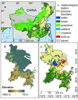
Yangtze River Delta is located in the middle of mainland coastline in Eastern China, where the Yangtze River empties into the ocean. This study area consists of southern Jiangsu Province, northern Zhejiang Province and Shanghai (Figure 1). The region is about 110,000 km2, across the east longitude from 116.8° to 124.2° and the north latitude from 26.99° to 34.64°, respectively. Yangtze River Delta belongs to the Middle-Lower Yangtze Plain, which is one of the China three Great Plains, with flat terrain. The agricultural lands are mainly distributed in the north and middle of this delta; the middle is Taihu River Basin with abundant water resources; the mountains and hills with lush vegetation cover the southwest region. This area is located in the subtropical monsoon climate zone with four distinct seasons, and has hot and humid summers, and cold and dry winters.
Figure 1. Location (a), DEM (b) and land cover/land use (c) maps
2.2 Data
2.2.1 MODIS data: The MODIS collection-5 products generated during 2012 provided by NASA were utilized in this study, including the daily LST product MYD11A1 (L3, 1 km), sixteen-day composite NDVI product MOD13A2 (L3, 1 km) and yearly land cover product MCD12Q1 (L3, 500 m). MYD11A1 is collected after radiometric calibration and atmospheric correction. And it has been verified that the data reliability below the 1000 meters above sea level reach up to 90 percent, and the accuracy is within 1 K (Wan et al., 2002). Two LST measurements are observed per day when Aqua transits along the equator at around 13:30 (day) and 1:30 (night) local time, which closely approximate the moments when daily minimum and maximum LST values occur. In order to ensure the uniformity of spatial resolution with LSTs, this paper adopted the IGBP classification scheme for the land cover product MCD12Q1, and resampled the spatial resolution from 500 meters to 1 kilometer. Note that in this study, we focus on the main types which mostly cover the Yangtze River Delta, and reduced the land cover types to six categories, including water, forest, grassland, wetland, cropland and built-up area (Figure 1c).
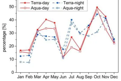
The presence of cloud cover in MODIS LST products, gives rise directly to the proportion of invalid data more than 60% in part of images, and affects the availability of LST data (Xu et al., 2010). In order to evaluate the monthly days under clear-sky condition in the study area in 2012, this paper calculated the average ratio of the clear-skies pixels to the total pixels for each month (Figure 2). As shown in Figure 2, the percentages in the spring (March, April, and May) and autumn (September, October, and November) are higher than that in summer (June, July, and August) and winter (January, February, and December) at different satellite observation time. Because the rainfall of Yangtze River Delta region is much abundant in summer, resulting in coverage by a large area of clouds. And the more clouds and haze directly reduce the amount of the data acquisition from satellites in winter (Huang et al., 2016).
Figure 2. Average percentage of clear-sky days during each month in 2012 for Yangtze River Delta
2.2.2 Meteorological data: The meteorological data of this paper are derived from the data of basic meteorological stations. Based on the daily meteorological data (including daily maximum and minimum AT) of 753 datum stations in China in 2012, the spatial interpolation using Inverse Distance Weighted (IDW) method was carried out to generate the daily maximum and minimum AT data with the spatial resolution of 500 meters. Among them, the Yangtze River Delta region contains a total of 23 datum stations (Figure 1c). In the process of temperature interpolation, taking into account the impact of the terrain elevation on temperature, that is, for every 1 kilometer above sea level rising, the temperature drops 6℃ (Liu et al, 2015). Then, the data of the Yangtze River Delta region were extracted from the national AT data, and the spatial resolution was resampled to 1 kilometer.
2.3 Method
2.3.1 Original ATC model: The ATC represents the variation of the daily average LST during a year. It is assumed that the patterns of temperature change in different seasons contain similar information under different insulation conditions. Therefore, several parameters which represent the overall trend of LST approximately during a year can be extracted from the variation (Bechtel, 2011). An ATC model described by a single sine function was used to fit the trend of daily average temperature over the course of a year (Bechtel, 2012; Zhan et al., 2014; Quan et al., 2016; Huang et al., 2016). As shown in Eq. (1).
2sin 365
d
f d MASTYAST
(1)
Where d is the day of the annual temperature cycle (relative to the spring equinox), and f d
represents the temperaturevalue corresponding to parameterd. MAST, YASTand are the key free parameters which determine the annual cycle for each pixel. MAST and YASTdenote the mean and amplitude of the temperature cycle during the year, and characterizes the phase displacement relative to the spring equinox. In this paper, the simple ATC model will be called the “Original Annual Temperature Cycle (ATCO) model”.
The basic principles of the ATC model are shown in Figure 3. It can be seen that the satellite observations of LST can’t be obtained for some days of the year due to the unclear-skies. Compared to the fluctuation of the real LSTs in the absence of cloud, a smooth curve is made up of the data simulated by ATC model.
Figure 3. A demonstration of the ATC model
2.3.2 Enhanced ATC model: Considering the differences between the curves of ATCO-based and real LSTs, this study developed a new ATC model based on ATCO model. Taking into consideration the synchronization relationship between daily mean LST variation and daily mean AT variation(Xu et al., 2010; Benali et al., 2012), incorporating the surface property information (e.g., NDVI), we improved the ability of the model for describing the short-term fluctuation of LSTs. The new model is referred to as the “Enhanced Annual Temperature Cycle (ATCE) model” in this work and can be described as follows:
2sin
365 a
d
f d MASTYAST T k'
(2)
max min
i min 1
NDVI NDVI
k' k
NDVI NDVI
(3)
Note that, the annual variation processes of each pixel are determined by four free parameters: the parameters MAST , YAST and are the same as those in the ATCO model; while the new parameter k is the coefficient that regulates the variation range of LST. These free parameters can quantitatively reflect the information of surface thermal characteristics, which is significant for the research of climate change and phenology. In Eq. (3), NDVIi represents the value of the NDVI for each
pixel on dayi. NDVImax and NDVImin denote the maximum NDVI and the minimum NDVI of a single pixel in a year, respectively. In addition, Ta is the difference between the
original AT values and the temperature data fitted by ATC model.
2.3.3 Sample and validation data: The LSTs of MYD11A1 product are utilized as the basic data to construct the ATC model in this work. Selected the clear-sky surface temperature data of MODIS at two time points of a day, 01:30 and 13:30 (when the Aqua LST are likely to be closer to the daily maximum and the minimum LST than that acquired from Terra, respectively (Coops et al., 2007)); explored the simulation effect on LST annual changes of the ATCE model during the day and night. During the process of selecting sample and validation data, 70 percent of the available LST data all through the year were randomly selected as the training samples, and the remaining 30 percent were used as validation data. In the course of training, the least squares method was adopted to solve the four parameters from the overdetermined equation. According to the key parameters, the simulated temperature can be determined at any time (day of year), and then compared with the verification data. The Root Mean Square Error (RMSE) was used to evaluate the error level, and quantitatively assessed the accuracy of the improved model.
3. RESULTS AND DISCUSSION
3.1 Analysis of RMSEs Distribution
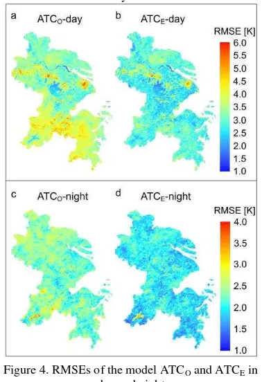
The simulation performance of the enhanced model has been presented by integrating the meteorological and NDVI data in the Yangtze River Delta region. Fig. 4 shows the spatial distribution of the RMSE of the model ATCO and ATCE during the day and night. As indicated in Figure 4a, the magnitude of the RMSEs in the study area varied greatly during the day. It is clear that the RMSEs in built-up area near the Yangtze River and Taihu Lake are the largest, mostly in the cities with fast economic growth and denser population, reaching the level of 6.0 K. Secondly, the study area has a higher terrain and mostly forest-covered areas, showing a large simulation error; while the minimum error of water area is to 1.5 K, such as the Yangtze River, Taihu Lake and Gaoyou Lake which is in the northern part of the study area, and the Thousand Island Lake which is in the south of the study area and so on. Compared to model ATCO, the simulation accuracy achieved by the model ATCE has significantly improved. The RMSE of decline level of the vegetation in the southern part of the study area is the largest and the error reduces to 2.5-3.5 K. The accuracy of the water area is not improved obviously, but the optimum accuracy level is maintained. However, some urban areas in Figure 4b, such as Shanghai, Nanjing, Changzhou and Wuxi, are still particularly prominent, and always maintain high RMSE values, about 4.0-5.0 K. There are two reasons for this: (1) In the LST data sets that have been acquired in a year, these pixels have a small number of anomalies that are much lower than the other data, resulting in larger errors in the pixels. It is analysed that these anomaly data result from the inversion’s error of MODIS LST data. (2) The numbers of available data for the pixels in different seasons are quite different. The observed data concentrate in spring and autumn, while lack long-term observation data in winter and summer because of the cloud cover and precipitation caused by the large heat cycle in the city, and that results in a large error in the simulated LST variation during the year. Figure 4c and 4d show the fit performance of two ATC models in the night. Unlike the RMSE Distribution in daytime, the results in night do not show correlations with the surface coverage types. Except the RMSE value of the Thousand Island Lake region of 3.5 K, the RMSEs of the model ATCO in the other regions are in the range of 2.0-3.0 K (Figure
4c). Figure 4d demonstrates that the model ATCE improves the
fitting accuracy (up to 1.5-2.5 K) for each region except the water body in the southern study area.
It is concluded that by comparing the degree of differences between the two models in daytime and night: by using the model ATCE to simulate the LST annual variation, the fitting accuracy has been improved on the whole, but there are great differences among different time periods and different land cover types. During the daytime, in most of the northern study area, the improvement degrees of accuracy are not obvious for around 0-0.5 K; the accuracy of the cultivated land in the south of the Yangtze River increases by about 0.7 K, and the simulation accuracy in the southern mountainous area are greatly improved for about 1.5 K. At night, the spatial distribution of the accuracy differences is similar to that of the daytime. The accuracies in most of the area are improved, especially in the mountainous area of Hangzhou with the RMSEs reduced by 1.0 K, except the water and some cultivated lands in the middle of the study area with value around 0 K.
Figure 4. RMSEs of the model ATCO and ATCE in day and night
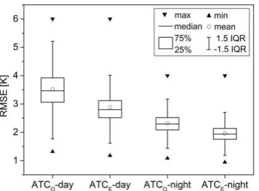
Figure 5 illustrates the diversities of RMSE values between model ATCO and ATCE from the perspective of error numerical distribution in day and night, respectively. In general, the mean RMSEs of model ATCO are 3.52 K and 2.32 K in day and night, while the values of model ATCE are 2.88 K and 1.96 K. Thus, the simulation precisions of day and night are increased by 0.64 K and 0.36 K. In the daytime, 21.1% of the values are concentrated in the range of 2.0-3.0 K for the original model, 57.0% in 3.0-4.0 K, and 18.6% in 4.0-4.0 K. And for the improved model, 2.5%, 64.8% and 28.1% of the values are concentrated in the ranges of 1.5-2.0 K, 2.0-3.0 K and 3.0-4.0 K. The distribution of the RMSEs of the two models at night is more concentrated than during the day: the initial model has values of 16.5% and 80.2% in 1.0-2.0 K and 2.0-3.0 K, respectively, while the improved model has values of 58.5% and 50.0% in the range of 1.0-2.0 K and 2.0-2.5 K, respectively.
Figure 5. Box charts showing the total RMSEs of model ATCO and ATCE. The end of each whisker indicates the highest or lowest value within 1.5 times the inter-quartile range (IQR)
Therefore, the model ATCE reduces the overall RMSEs compared to ATCO in the process of fitting LST annual variations. The concentrated numerical distribution and the better improvement level of accuracy in the daytime than that in the night, demonstrate the inference that the new model has better performance. In addition, it can be seen from Figure 4
and Figure 5 that the ATC model has a poorer ability on the simulation of LST annual variation during daytime, and the RMSEs are smaller at night. From the perspective of the ATC model, it may be affected by solar radiation. For the same place at the same time each day, the LST changes more strongly during the day. The time of daily LSTs observed by satellites is changing (not always at 13:30), so that the differences of LSTs are affected by the time changes in the range of two hour. Besides, the precipitation or other weather changes directly disturb the regular variations of LSTs, resulting in greater differences of the satellite observation time have a less influence on the ATC model. Therefore, the LST annual variation tends to be a sinusoidal function for the better performance.
3.2 RMSEs of different Land cover types
The Yangtze River Delta was divided into six different land cover types by using the NDVI data. Table 1 displays the average RMSEs of the pixels under the coverage of various types, that quantitatively analyse the similarities and differences of simulation capabilities between the pixels in various land cover types with the improved ATC model.
Land cover
Table 1. RMSEs of model ATCE in different land cover types
By analysing the RMSEs of various ground types based on the ATCO model during the day, it is concluded that the RMSEs of built-up, forest and grassland areas are larger than 3.5 K, while water area is the lowest with the RMSE of 2.50 K. Improved by
the ATCE model, the RMSE of the forest decreased by about improved significantly. Because of the larger specific heat capacity, the water is less affected by clouds, precipitation and other weather changes, and it gives rise to similar simulation results of the water temperature based on two models. For other types of pixels, such as grassland, crop land and built-up areas, there are faster responses reflected in LSTs to the weather changes, especially in built-up area where the temperature of impervious layer changes rapidly with the process of precipitation. Consequently, the temperatures of such kinds of surface displayed more complex fluctuations over a year, which increased the difficulties of fitting with regular mathematical models, resulting to relatively poorer simulation effect. At night, the RMSEs of all land cover types based on the ATCO model reflect the similar pattern with the values between 2.26 and 2.34 K. and the accuracies based on the ATCE model are improved to 2.0 K.
As indicated in Table 1, the deviations of fitting effects based on model ATCE between the daytime and nighttime on the land types are different except for water area, while especially inbuilt-up, forest and grassland areas with the deviation over 1.0 K. It implies that, the stability of the experimental data directly affects the effects of model. The greater stability of the data, the better results will be simulated. From the above, for all land covers, the ATCE model with the temperature data as an auxiliary factor effectively described the variation of LST fluctuations. method, the maps of spatial distribution of seasonally mean LST differences in four seasons (divided March, April, May into spring; June, July, August into summer; September, October, November into autumn; December, January and February into winter) based on two ATC models are presented in Figure 6. In these figures, if the differences are more than 0 K, it means that the LST values estimated by the ATCO model at the pixel are larger than the values generated by the ATCE model.
It is provided in Figure6a that in spring, the values range from -0.3 to 1.0 K. Near the Taihu Lake and the crop lands in north of this study area, the values approximately equal 0 K, but the differences in forest and built-up areas are around 1.0 K, especially in Nanjing and Shanghai with the maximum value about 1.5 K. In summer, 98.8% of the values are greater than 0 K except for some coastal cities, and the differences in the southern part of the study area covered by mountains are over 3.0 K. The range of values for the whole study area is from -1.5 to 0.5 K in autumn and 94.4% of the values are negative. It can particularly be observed in higher ground, such as Nanjing, Shanghai and the southwest of the Taihu Lake. With the similar spatial pattern to spring, the range of values in winter is between -1.5 K and 3.0 K. But the difference is the larger
values in southern study area, and the value in Shaoxing reaches the top of 3.0 K. It can be seen that there are large differences between the two models in estimating the mean LST values in summer and winter, with the absolute value over 3.0 K, while in spring and autumn are slighter within 1.5 K. Besides, the LSTs estimated by ATCO are larger than that by ATCE in spring and summer, while the differences are the opposite in autumn, and the values in winter change with the types of land covers.
Figure 6. Map of LST differences in seasons between model ATCO and ATCE
Figure 6b illustrates the differences between the nights. The values of the water and the forests in southeastern study area are less than 0 K in spring and the rest of the area reach 0.5 K. The differences in autumn are generally lower than 0 K, ranging from -1.0 K to 0 K. For summer and winter, the deviations are more than 0 K, and those of the southern mountain area in summer and the crop land in north of the Yangtze River in winter get the greater value over 1.5 K. It can also be found that the phenomenon similar to the daytime: the differences in
summer and winter (over 2.0 K) are greater than that in spring and autumn (around 0.5 K).
3.4 Discussion related to temporal upscaling
The daily LST data in a year were estimated with ATCE model using the observed LST data, and established the LST annual variation curve. However, due to the different amount of LST data in different clear seasons, the spring and autumn seasons are more concentrated and the summer and winter seasons are more sparse, which leads to the uneven distribution of the model data, which affects the accuracy of simulating real LSTs. Here, we carried out experiments: the observed LST in 2012, the time series were divided to 1, 2, 4, 8, 16 and 32 days for the temporal synthesis (Huang et al., 2016). Then use the synthetic data to set up ATCE model, and calculate the RMSEs between the annual variation and observed data of surface temperature.
Figure 7 is the RMSEs plot of the ATCE model for multi-time synthesis scales. It can be seen from the figure that the simulation error of the ATCE model in the daytime and nighttime show a decreasing trend with the increase of the time synthesis unit. At different time scales, the errors during the day are greater than the night, and the decreasing amplitude of RMSE during the day is also larger than the night. In the daytime, the RMSE of the model is 2.9 K when the time unit is 1 day, and the precision is about 1.8 K when the time unit adds to 32 days. And the decrease of RMSE is about 1.0 K. At night, the RMSE was 1.9 K and 1.3 K at 1 and 32 days, respectively, with the difference of 0.6 K.
Figure 7. RMSEs of ATCE model in multi-time synthesis scales
It is shown that the precision of the ATCE model is improved by the data processing method of temporal upscaling, which neglects the data points where the LSTs changes rapidly within the temporal synthesis unit. However, the temporal upscaling method is suitable for the study of the monthly variation of surface temperature, while the LST data of “day” is still needed to study the annual variation trend of surface temperature.
4. CONCLUSIONS
This study devised ATCE model to reconstruct consistent, daily LSTs based on ATCO model by using MODIS products. It is effective in improving the accuracy of ATC model by considering the impact of air temperature on the LST variation combined with NDVI information. Compared to the model ATCO, the simulation accuracy of model ATCE improved by 0.64 K and 0.36 K in daytime (13:30 at local time) and night time (1:30 at local time), respectively. Due to the larger change of LST-observed in the daytime and the stable change of the
night over a year, the ATC model has a better performance for fitting LST annual variation during the night. It was found that the improvements of accuracies varied with different land cover types: the forest, grassland and built-up areas improved larger than water area. In addition, the spatial heterogeneity was observed for performance of ATC model on different land covers: the RMSEs of built-up area, forest and grassland were larger than 3.5 K in the daytime, while the water attained the best performance with 2.50 K; at night, the accuracies of all land cover types significantly increased to similar level with RMSE around 2 K. Furthermore, by comparing the differences between LSTs simulated by two models in different seasons, it was found that the differences were smaller in the spring and autumn, while larger in the summer and winter.
It was presented that, the data sets observed at different time scales have a significant effect on the accuracy of the ATCE. The less data gaps occur in the time series, the more uniform the data distribute, and the higher accuracy the model reaches. From the “day” to “month”, the simulation RMSEs of the ATCE model in the daytime and night time showed a decreasing trend with the increase of the temporal synthesis unit. Therefore, it is important to think about the effect of time scales before applying the ATC model.
Although progress in understanding the ATC model has been made, there remain uncertainties that will become the focus of future research. The four parameters is the core of the ATC model, although the parameters are calculated by the least squares algorithm, there are still certain deviations (e.g., deviation caused by the uneven distribution of data with the process of solving parameters), and result in the large errors of the ATC model in some areas. Moreover, in order to expand the applications of the ATC model, the more extensive research in more land cover types, such as snow and desert areas, should be carried out.
REFERENCES
Bechtel, B., 2011. Multi-temporal Landsat data for urban heat island assessment and classification of local climate zones. Urban Remote Sensing Event, pp. 129 - 132.
Bechtel, B., 2012. Robustness of annual cycle parameters to characterize the urban thermal landscapes. IEEE Geoscience and Remote Sensing Letters, 9(9), 876-880.
Benali, A., Carvalho, A. C., Nunes, J. P., Carvalhais, N., Santos, A., 2012. Estimating air surface temperature in portugal using modis lst data. Remote Sensing of Environment, 124(9), 108-121.
Coops, N.C., Duro, D.C., Wulder, M.A., Han, T., 2007. Estimating afternoon MODIS land surface temperatures (LST) based on morning MODIS overpass, location and elevation information. International Journal of Remote Sensing, 28: 2391-2396.
Crosson, W.L., Al-Hamdan, M.Z., Hemmings, S.N., Wade, G.M., 2012. A daily merged MODIS Aqua–Terra land surface temperature data set for the conterminous United States. Remote Sensing of Environment, 119: 315-324.
Dickinson, R.E., Henderson-Sellers, A., Kennedy, P. J., Atmospheric, N. C. F., 1993. Biosphere-atmosphere transfer scheme(BATS) version 1e as coupled to the NCAR community
climate model. National Center for Atmospheric Research, Climate and Global Dynamics Division.
Duan, S.B., Li, Z.L., Wu, H., Tang, B.H., Jiang, X.G., Zhou, G.Q., 2013. Modeling of day-to-day temporal progression of clear-sky land surface temperature. IEEE Geoscience and Remote Sensing Letters, 10: 1050-1054.
Fu, P., Weng, Q.H., 2016. Consistent land surface temperature data generation from irregularly spaced landsat imagery. Remote Sensing of Environment, 184, 175-187.
Giglio, L., Descloitres, J., Justice, C. O., Kaufman, Y. J., 2003. An Enhanced Contextual Fire Detection Algorithm for MODIS. Remote Sensing of Environment, 87, 273-282.
Göttsche, F.M., Olesen, F. S., 2001. Modelling of diurnal cycles of brightness temperature extracted from METEOSAT data. Remote Sensing of Environment, 76, 337-348.
Göttsche, F.M., Olesen, F.S., 2009. Modelling the effect of optical thickness on diurnal cycles of land surface temperature. Remote Sensing of Environment, 113: 2306-2316.
Huang, F., Zhan, W.F., Duan, S.B., Ju, W., Quan, J.L., 2014. A generic framework for modeling diurnal land surface temperatures with remotely sensed thermal observations under clear sky. Remote Sensing of Environment, 150(7), 140-151.
Inamdar, A.K., French, A., Hook, S., Vaughan, G., Luckett, W., 2008. Land surface temperature retrieval at high spatial and temporal resolutions over the southwestern United States. Journal of Geophysical Research, 113: D07107.
Jiang, G.M., Li, Z.L., Nerry, F., 2006. Land surface emissivity retrieval from combined mid-infrared and thermal infrared data of MSG-SEVIRI. Remote Sensing of Environment, 105: 326-340.
Ke, Y.E., Qin, Z.H., 2006. A study of urban heat island in summer of nanjing based on modis data. Remote Sensing Technology and Application, 21(5), 426-431.
Liu, Y., Xiao, J., Ju, W., Zhou, Y., Wang, S., Wu, X., 2015. Water use efficiency of china’s terrestrial ecosystems and responses to drought. Scientific Reports, 5(5), 13799.
Metz, M., Rocchini, D., Neteler, M., 2014. Surface temperatures at the continental scale: tracking changes with remote sensing at unprecedented detail. Remote Sensing, 6(5), 3822-3840.
Quan, J.L., Zhan, W.F., Chen, Y.H., Wang, M., Wang, J., 2016. Time series decomposition of remotely sensed land surface temperature and investigation of trends and seasonal variations in surface urban heat islands. Journal of Geophysical Research Atmospheres, 121(6), n/a-n/a.
Ramsey, M.S., Harris, A.J.L., 2013., Volcanology 2020: How will thermal remote sensing of volcanic surface activity evolve over the next decade? Journal of Volcanology and Geothermal Research, 249, 217-233.
Sagalovich, V.N., Fal'kov, E.Y., Tsareva, T.I., 2002. Determination of diurnal soiltemperature cycles using remote sensing data. Mapping Sciences and Remote Sensing, 39: 46-55.
Schädlich, S., Göttsche, F.M., Olesen, F.S., 2001. Influence of land surface parameters and atmosphere on METEOSAT brightness temperatures and generation of land surface temperature maps by temporally and spatially interpolating atmospheric correction. Remote Sensing of Environment, 75: 39-46.
Sobrino, J.A., El Kharraz, M.H., 1999a. Combining afternoon and morning NOAA satellites for thermal inertia estimation: 1. Algorithm and its testing with Hydrologic Atmospheric Pilot Experiment‐Sahel data. Journal of Geophysical Research, 104: 9445-9453.
Sobrino, J.A., El Kharraz, M.H., 1999b. Combining afternoon and morning NOAA satellites for thermal inertia estimation: 2. Methodology and application. Journal of Geophysical Research, 104: 9455-9465.
Van den Bergh, F., van Wyk, M.A., van Wyk, B.J., 2006. Comparison of datadriven and model-driven approaches to brightness temperature diurnal cycle interpolation. In, 17th Annual Symposium of the Pattern Recognition Association of South Africa. Parys, South Africa.
Voogt, J.A., Oke, T.R., 2003. Thermal remote sensing of urban climates. Remote Sensing of Environment, 86, 370-384.
Wan, Z.M., Li, Z.L., 1997. A physics-based algorithm for retrieving land-surface emissivity and temperature from eos/modis data. IEEE Transactions on Geoscience and Remote Sensing, 35(4), 980-996.
Wan, Z.M., Zhang, Y., Zhan, Q., Li, Z.L., 2002. The MODIS Land-Surface Temperature products for regional environmental monitoring and global change studies. In Geoscience and Remote Sensing Symposium, 2002.IEEE International, Vol. 6, pp. 3683-3685.
Wang, Y., 2011. Regional representativeness analysis of national reference climatological stations based on modis/lst product. Journal of Applied Meteorological Science, 22(2), 214-220.
Watson, K., 2000. A diurnal animation of thermal images from a day–night pair. Remote Sensing of Environment, 72: 237-243.
Wu, L.X., Qin, K., Liu, S.J., 2012. GEOSS-based thermal parameters analysis for earthquake anomaly recognition. Proceedings of the IEEE, 100, 2891-2907.
Xu, Y., Qin, Z.H., Shen, Y., 2010. The relationship between inter-annual variations of land surface temperature and climate factors in the yangtze river delta. Remote Sensing for Land and Resources, 27(1), 60-64.
Xu, Y., Shen, Y., 2013. Reconstruction of the land surface temperature time series using harmonic analysis. Computers and Geosciences, 61, 126-132.
Zhan, W., Chen, Y., Zhou, J., Wang, J., Liu, W., Voogt, J., et al., 2013. Disaggregation of remotely sensed land surface temperature: literature survey, taxonomy, issues, and caveats. Remote Sensing of Environment, 131(8), 119-139.
Zhan, W.F., Zhou, J., Ju, W.M., Li, M.C., Sandholt, I., Voogt, J., Yu, C., 2014. Remotely sensed soil temperatures beneath snow-free skin-surface using thermal observations from tandem
polar-orbiting satellites: An analytical three-time-scale model. Remote Sensing of Environment, 143, 1-14.
Zhao, W., Li, Z.L., Wu, H., Tang, B.H., Zhang, X., Song, X., et al., 2013. Determination of bare surface soil moisture from combined temporal evolution of land surface temperature and net surface shortwave radiation. Hydrological Processes, 27(19), 2825–2833.