*Corresponding author.
E-mail addresses:[email protected] (M.F. Gorman), [email protected] (J.I. Brannon)
Seasonality and the production-smoothing model
Michael F. Gorman
!
, James I. Brannon
"
,
*
!Department of Operations Research, Burlington Northern Santa Fe Railway, USA "Department of Economics, University of Wisconsin Oshkosh, Oshkosh, WI 54901, USA
Received 20 June 1996; accepted 25 January 1999
Abstract
The debate over whether"rms smooth production relative to demand continues. In this paper we"nd that results
obtained in Blinder (Quarterly Journal of Economics 101 (3) (1986) 431}453) and Blinder and Maccini (Journal of
Economic Surveys 5 (4) (1991) 293}328), indicating that"rms do not smooth production, are greatly in#uenced by the
seasonal adjustment of the Census data for US manufacturing. Using seasonally adjusted data, we "nd signi"cant
evidence of production smoothing in 10 of 14 manufacturing industries for the years 1982}1997. Further, the prevalence
of production smoothing has increased over time, which we attribute either to fundamental changes in the collection of
the data or to the advent of improved methods of inventory management. ( 2000 Elsevier Science B.V. All rights
reserved.
Keywords: Inventory; Backorder; Production-smoothing; Seasonal adjustment
1. Introduction
The main goal of the production-smoothing literature has been to discern the extent to which
"rms use inventories to smooth production levels
in the face of #uctuating demand. Whether "rms
smooth or bunch production over time is not merely an academic question; it has broad implica-tions for the business cycle, inventory demand and even seasonal and frictional unemployment.
Others have shown that seasonally unadjusted data are preferable to seasonally adjusted data
when doing dynamic production studies [1}3].
Nevertheless, studies have typically used seasonally
adjusted data to characterize dynamic"rm
behav-ior [4,5]. Through a direct comparison of sea-sonally adjusted and unadjusted Census data, we show that seasonally unadjusted data manifest the
production-smoothing behavior of "rms more
accurately than seasonally adjusted data.
When measuring the extent of production smoothing, seasonally unadjusted data have two
advantages. First, seasonal #uctuations comprise
the largest source of the#uctuations in inventory,
production and shipments series, so seasonal ad-justment reduces the ability to estimate the extent
of the production smoothing e!ect of inventories.
Second, seasonal #uctuations are regular,
an-ticipated and short-lived, the type of #uctuation
over which a"rm is most likely to use inventories
to smooth production. Business cycle#uctuations
have a much more uncertain length and depth and produce inventory changes that cannot be
sus-tained inde"nitely; production adjustments follow
and inventories fail to act as a bu!er.
Our results show that the seasonal adjustment of data alters the perceived relationship between the
production, shipments and "nished goods
inven-tory variables and produces misleading results in
tests of production smoothing. We"nd that while
seasonally adjusted data indicates production is more variable than shipments, indicating no pro-duction smoothing, seasonally unadjusted data
shows that production is less variable than
ship-ments in 10 of 14 manufacturing industries. We conclude that only seasonally unadjusted data should be used for studies of dynamic production behavior.
2. Literature review
Blinder [4] and Blinder and Maccini [6] "nd
little evidence to support the production-smooth-ing hypothesis. Usproduction-smooth-ing monthly, seasonally adjusted data for durable and nondurable manufacturing
from the Census Bureau, the two studies"nd the
ratio of the variance of production to the variance of shipments falls between 1.03 and 1.20 for the two sectors and the covariance of shipments and change in inventories to be positive. For two-digit SIC industries, the ratio ranges from 0.93 to 1.38, with 17 out of 20 industries having a ratio greater than one. A ratio of the variances of production and shipments less than one strongly supports the pro-duction-smoothing hypothesis.
In light of the paucity of evidence supporting production smoothing, researchers responded by attempting to refute the very idea of production smoothing. Production smoothing may not exist, it has been suggested, due to the stochastic behavior of demand, concavity of costs and the existence of
signi"cant supply shocks in manufacturing.
Researchers have also tried to"nd new ways of
testing the production-smoothing hypothesis, fo-cusing on the properties of the data used to test the hypothesis. For instance, there might be a positive correlation between inventories and sales due to the behavior of demand shocks and the
develop-ment of expectations. Blinder [4] suggests that if
a motivation for inventories is to avoid un"lled
orders, then desired inventories are a positive func-tion of current and future expected sales. In
adjust-ment to expectations,"rms accumulate inventories
even in the face of increased sales.
Ramey [7] argues that manufacturers face
con-cave costs, owing to"rms'incentive to build excess
capacity and hoard labor during low production periods. Further, Ramey suggests that concave costs of adjustment contribute to the explanation of production-bunching behavior. The problems of rebalancing assembly lines when changing output levels in capital-intensive production industries may lead to large shifts in output rather than grad-ual transitions from one level to the next.
Alternatively, cost shocks through time could
cause "rms to over-produce during low-cost
periods and under-produce in high-cost periods. Blinder [4] and West [8] note that if cost shocks play a larger role in production decisions than
demand shocks, then"rms could optimally bunch
production. Blinder [4] doubts that cost shocks dominate demand shocks in the macroeconomy, but combined with the serial correlation of demand
shocks, the two e!ects could produce production
bunching.
Ray Fair [1] suggests the failure of the produc-tion smoothing model arises from the problems of the Census data used by Blinder [4] and Blinder
and Maccini [5] and others to describe"rm
behav-ior. Using physical unit data for various three-digit
SIC industries, Fair "nds strong support for
pro-duction smoothing. Miron and Zeldes [2] as well
as Krane and Braun [9] support this story,"nding
signi"cant di!erences between Census data and
indices of production from the Federal Reserve. However, Blanchard [10] reports evidence to the contrary using physical data from the US auto-mobile industry.
Ghali [3] shows seasonal adjustment a!ects
production-smoothing results. His data from the Portland cement industry supports production smoothing only in data that are not seasonally adjusted; after seasonal adjustment, he obtains
re-sults similar to Blinder's. Miron and Zeldes [2] also
recognizes the importance of using seasonally
1Monthly is the greatest frequency reported; time aggregation can obscure the inventory}production relationship.
2Until 1982,"rms were asked to report their inventories at book values, according to whatever method they used for tax purposes (LIFO, FIFO, and so forth). Because of this, the value of aggregate inventories for an industry was not precise. E! ec-tive with the 1982 Census of Manufactures, instructions for reporting inventories changed. LIFO users were asked to report inventories prior to the LIFO adjustment, as well as the LIFO reserve and the LIFO value after adjustment for the reserve. (From the Manufacturers'Shipments, Inventories, and Orders (M3) Survey.)
of production smoothing of seasonal and
non-seasonal#uctuations for various two-digit SIC
in-dustries.
Ghali and Dimelis [11], using data for six highly
disaggregated industries from 1950 to 1960, "nd
signi"cant evidence of production smoothing either
using the variance bounds test or estimating a re-duced form equation. They suggest that the failure of previous models to detect production smoothing is either due to the level of aggregation or the test used.
3. Data
We have monthly, seasonally adjusted and unad-justed data on production, inventory, shipments and new orders from 1959 to 1997 for 14 2-digit SIC industries in both durable and nondurable manufacturing. We also have the same aggregate data for durable, nondurable and total
manufactur-ing.1All but the production series comes from data
"les supplied by the Census Bureau; production numbers were created from the identity
P
t,St#(Ft!Ft~1), (1)
whereP
tis the production in periodt,Stthe
ship-ments in periodt, andF
tthe inventory at the end of
periodt.
Because of their intertemporal nature,
invento-ries cannot be properly de#ated by a simple index.
We calculate real values by considering both cur-rent and lagged price levels, as well as the age composition of the goods held in inventory. To
de#ate nominal seasonally unadjusted data we
cal-culated the implied de#ator of the BEA for
sea-sonally adjusted inventories from the ratio of nominal and real seasonally adjusted inventory numbers [2]. As in West [8], inventory numbers are converted from cost to market values by an
industry-speci"c factor in order to adjust for the
ratio of shipments to cost of goods sold.
Due to a change in inventory recording methods by the Census bureau in 1982, the inventory
num-bers from before and after that time are not consis-tent. Thus, we separate our data analysis into pre-1982 and post-1982 results, placing more weight on the latter simply because the revision in
the data collection appears to have signi"cantly
improved the reliability of the data.2
4. Seasonally adjusted vs. unadjusted data comparisons
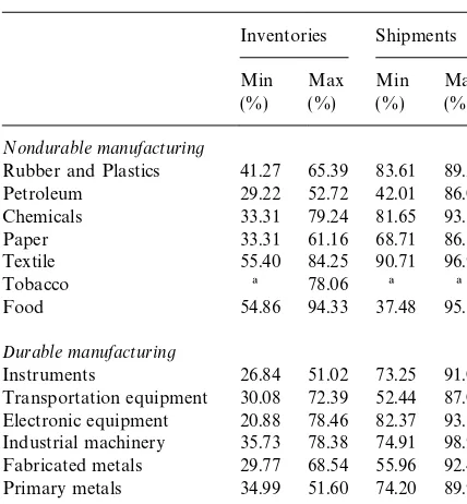
Our"rst task is to demonstrate that seasonality is indeed important in the behavior of variables relevant to production smoothing. This is easily achieved by examining Table 1, taken from the
1998 Current Industrial Reports, M3-1 (95). Table 1 compiles data from Appendix E (M3-1 [95]) of the
report, which details the monthly #uctuations in
inventories and shipments, the variables that sum to production. It reports the maximum and
min-imum proportion of the monthly #uctuations
at-tributable to seasonal factors for 14 2-digit SIC
variables. It shows that seasonal #uctuations are
almost always the major source of variance in every single variable we examine, sometimes causing as much as 98% of the total variability in inventory or shipments. Table 1 succinctly illustrates our point that using seasonally adjusted data when testing for production-smoothing behavior obscures the most
important cause of demand#uctuations.
Figs. 1 and 2 also demonstrate the importance of
seasonality as a source of#uctuations. Figs. 1 and 2
show the #uctuations in durable goods
Table 1
Seasonality's e!ect on inventory and shipment time series per-cent of total variation attributable to seasonality from Appendix G,Current Industrial Reports
Inventories Shipments
Min Max Min Max
(%) (%) (%) (%)
Nondurable manufacturing
Rubber and Plastics 41.27 65.39 83.61 89.28
Petroleum 29.22 52.72 42.01 86.07
Chemicals 33.31 79.24 81.65 93.51
Paper 33.31 61.16 68.71 86.19
Textile 55.40 84.25 90.71 96.93
Tobacco ! 78.06 ! !
Food 54.86 94.33 37.48 95.33
Durable manufacturing
Instruments 26.84 51.02 73.25 91.08
Transportation equipment 30.08 72.39 52.44 87.09 Electronic equipment 20.88 78.46 82.37 93.15 Industrial machinery 35.73 78.38 74.91 98.98 Fabricated metals 29.77 68.54 55.96 92.44 Primary metals 34.99 51.60 74.20 89.95 Stone, clay and glass 47.87 71.31 85.13 90.60 !Not reported.
Consistent with Blinder [4] and Blinder and Maccini [5], we measure the extent of production smoothing by examining the ratio of the variance of
production to the variance of shipments for a"rm
or industry. Table 2 provides the variance ratios for 14 2-digit SIC manufacturing industries and for total, durable, and non-durable manufacturing, cal-culated for both seasonally adjusted and unadjus-ted data. This method is intuitively appealing; a ratio less than one indicates that output changes less than shipments and hence inventories are being used to smooth production.
Neither Blinder nor Blinder and Maccini "nd
much evidence of production smoothing using sea-sonally adjusted data; Blinder estimated a variance ratio of 1.20 for DUR and 1.05 for NDUR; Blinder and Maccini obtained 1.03 for both sectors with
a slightly larger data set. We"nd similar results for
seasonally adjusted data regardless of the industry, aggregation, or time frame, with only 1 industry (primary metals) showing any evidence of
produc-tion smoothing. Of course, as we argued before,
there is no reason for there to be signi"cant
produc-tion smoothing outside of the seasonal demand
#uctuations.
However, using seasonally unadjusted data, we
"nd abundant evidence of production smoothing.
Using the more reliable post-1982 data we"nd the
variance ratios to be below 1 in 10 of the 14 indus-tries, as well as in aggregate non-durable, durable, and total manufacturing. Correcting for the impre-cise pre-1982 numbers and the seasonal adjust-ment, the data give the unmistakable impression that production smoothing occurs to some degree in most manufacturing industries. It is not surpris-ing that Blinder did not detect evidence of produc-tion smoothing in his data; as we point out,
seasonal#uctuations are the source of most of the
variability in demand.
In general, seasonally unadjusted data and
sea-sonally adjusted data provide signi"cantly di!erent
answers to the question of production smoothing. We"nd strong support for the production-smooth-ing hypothesis usproduction-smooth-ing seasonally unadjusted data, particularly in post-1982 data.
5. Conclusion
This paper supports the production-smoothing
hypothesis. While Blinder's seminal work in the
area fails to detect any evidence of production smoothing, merely using seasonally unadjusted
data and updating the data set reverses his"nding.
Since we show that seasonal factors are the primary
source of #uctuations in output, we argue that
ignoring such factors by using seasonally adjusted data is inappropriate.
Our results complement Ghali [3] and Dimelis
and Ghali [11], which"nd evidence of production
smoothing for a small number of highly disag-gregated industries in an earlier time period. Thus, our work suggests that production smoothing is a somewhat robust result that is solely dependent upon using seasonally unadjusted data.
The results have implications for any study of
dynamics; seasonal #uctuations have signi"cant
Fig. 1. Durable good shipments for seasonally adjusted and seasonally unadjusted goods.
Fig. 2. SA and NSA total manufacture"nished goods inventory 1990}1998.
Table 2
Var(production)/Var(shipments) for seasonally adjusted (SA) and seasonally unadjusted (NSA) data 1958}1998
Industry Pre-1982 Post-1982
SA NSA SA NSA
Total manufacturing 1.05 1.02 1.08 0.78 Nondurable manufacturing 1.34 1.08 1.04 0.81 Rubber and plastics 1.66 1.23 1.38 1.04
Petroleum 1.38 1.40 1.73 1.44
Chemicals 1.39 0.82 1.87 0.80
Paper 1.37 1.01 1.66 1.04
Textile 1.40 1.10 1.79 0.87
Tobacco 4.10 14.93 0.73 0.44
Food 1.35 1.15 1.08 0.73
Durable manufacturing 1.01 1.01 1.24 0.81
Instruments 2.43 1.08 1.88 0.77
Transportation equipment 1.04 0.93 1.24 0.93
Electronics 1.55 1.14 2.43 0.74
Industrial and mach. equip. 1.43 1.11 3.08 0.70 Fabricated metals 1.57 1.21 1.69 1.12
Primary metals 0.83 0.90 0.96 0.94
Stone, clay and glass 1.52 0.84 1.09 0.83
When there are short term, fairly predictable
changes in output demand, as we "nd in seasonal
cycles, it is only natural for "rms to respond by
using inventories as a bu!er. For less predictable
output demand#uctuations,"rms may be less apt
to respond with inventory, but may simply choose
not to"ll all orders.
A more highly disaggregated data set covering more industries might allow the researcher to
dis-cern the extent to which inventories and un"lled
Acknowledgements
Thomas Kniesner, Benjamin Craig, John Muth and two anonymous referees provided helpful com-ments on earlier drafts, and Jennifer Ribarsky assisted with the data collection.
References
[1] R. Fair, The production smoothing model is alive and well, Working Paper, No. 2877, March, National Bureau of Economic Research, Cambridge, MA, 1989.
[2] J.A. Miron, S.P. Zeldes, Seasonality, cost shocks, and the production smoothing model of inventories, Econometrica 56 (1988) 877}908.
[3] M.A. Ghali, Seasonality, aggregation and the testing of the production smoothing hypothesis, American Economic Review 77 (3) (1987) 464}470.
[4] A.S. Blinder, Can the production smoothing model of inventory behavior be saved? Quarterly Journal of Econ-omics 101 (3) (1986) 431}453.
[5] A.S. Blinder, L.J. Maccini, Taking stock: A critical assess-ment of recent research on inventories, Journal of Eco-nomic Perspectives 5 (1) (1991) 73}96.
[6] A.S. Blinder, L.J. Maccini, The resurgence of inventory research: What have we learned? Journal of Economic Surveys 5 (4) (1991) 293}328.
[7] V.A. Ramey, Nonconvex costs and the behavior of inventories, Journal of Political Economy 99 (1991) 306}333.
[8] K.D. West, A variance bounds test of the linear quadratic inventory model, Journal of Political Economy 94 (1986) 374}401.
[9] S. Krane, S. Braun, Production smoothing: Evidence from physical product data, Board of Governors of the Federal Reserve System, Washington, DC, June 1989.
[10] O.J. Blanchard, The production and inventory behavior of the American automobile industry, Journal of Political Economy 91 (1983) 365}400.