Full Terms & Conditions of access and use can be found at
http://www.tandfonline.com/action/journalInformation?journalCode=ubes20
Download by: [Universitas Maritim Raja Ali Haji] Date: 12 January 2016, At: 23:07
Journal of Business & Economic Statistics
ISSN: 0735-0015 (Print) 1537-2707 (Online) Journal homepage: http://www.tandfonline.com/loi/ubes20
Improved Errors-in-Variables Estimators for
Grouped Data
Paul J Devereux
To cite this article: Paul J Devereux (2007) Improved Errors-in-Variables Estimators for Grouped Data, Journal of Business & Economic Statistics, 25:3, 278-287, DOI: 10.1198/073500106000000189
To link to this article: http://dx.doi.org/10.1198/073500106000000189
Published online: 01 Jan 2012.
Submit your article to this journal
Article views: 115
View related articles
Improved Errors-in-Variables Estimators
for Grouped Data
Paul J. D
EVEREUXSchool of Economics, UCD Dublin, Belfield, Dublin 4, Ireland (devereux@ucd.ie)
Grouping models are widely used in economics but are subject to finite sample bias. I show that the stan-dard errors-in-variables estimator is exactly equivalent to the jackknife instrumental variables estimator and use this relationship to develop an estimator which, unlike the standard errors-in-variables estimator, is unbiased in finite samples. The theoretical results are demonstrated using Monte Carlo experiments. Finally, I implement a model of intertemporal male labor supply using microdata from the U.S. Census. There are sizable differences in the wage elasticity across estimators, showing the practical importance of the theoretical issues even when the sample size is quite large.
KEY WORDS: Labor supply; Pseudo-panel; Small-sample bias.
1. INTRODUCTION
In many economic applications, observations are naturally categorized into mutually exclusive and exhaustive groups. For example, individuals can be classified into cohorts, and workers are employees of a particular firm. The simplest grouping esti-mator involves taking the means of all variables for each group and then carrying out a group-level regression by ordinary least squares (OLS) or weighted least squares (if there are differ-ent numbers of observations in differdiffer-ent groups). This estimator has been called the efficient Wald estimator (Angrist 1991). For brevity, I refer to it as EWALD in this article. Grouping esti-mators have been used in recent years to study labor supply (Angrist 1991; Blundell, Duncan, and Meghir 1998; Devereux 2004), consumption (Mckenzie 2001), wage inequality (Card and Lemieux 1996), intergenerational transfers of human capi-tal (Acemoglu and Pischke 2001), and many other topics.
Deaton (1985) pointed out that EWALD is biased in finite samples and proposed an errors-in-variables estimator (EVE) to correct for the effects of sampling error. The first contribution of this article is to analyze the relationship between errors-in-variables estimators and bias-corrected instrumental errors-in-variables estimators. These two types of estimators have been developed in separate literatures and, to my knowledge, the relationships between them have not been studied in either literature. I show that, in the grouping context, EVE is exactly equivalent to the jackknife instrumental variables estimator (JIVE) of Phillips and Hale (1977), Angrist, Imbens, and Krueger (1995, 1999), and Blomquist and Dahlberg (1994, 1999). The relationship be-tween EVE and thek-class of instrumental variables estimators is also developed.
The second contribution of this article is to use the equiva-lence of EVE and JIVE to examine the small-sample bias of EVE and to develop an errors-in-variables estimator (UEVE) that is approximately unbiased. Unlike many instrumental vari-ables estimators, UEVE can be implemented in situations where the microdata are unavailable provided estimates of the variance of sampling errors can be obtained. The theoretical re-sults are supported by Monte Carlo evidence that EVE often has substantial biases but UEVE is close to unbiased and tends to have lower finite sample variance than EVE. In the final section of the article I estimate a model of intertemporal labor supply using a cohort approach in repeated cross-sectional data. There are sizable differences in the wage elasticity across estimators,
showing the practical importance of the theoretical issues dis-cussed in this article even in circumstances where the sample size is quite large.
2. THE GROUPING MODEL
Assume that there areGgroups andngis the number of ob-servations in groupg. The sample mean ofx for groupg,xg, is the mean ofx over all members of groupgincluded in the sample. The population mean ofx for that group(πg)relates to the mean ofxfor all members of the underlying population who are in that group. Consider the following model:
ygi=π′gβ+ugi, i=1, . . . ,ng,g=1, . . . ,G, (1) xgi=πg+vgi. (2) Hereπgandβ are K×1 vectors, whereK is the number of right-side variables andGg=1ng=N.
Taking means within groups,
yg=π′gβ+ug, (3) xg=πg+vg. (4) Assume that the sampling error has the following structure:
ug vg
∼iid
0, 1
ng
̺ σ′
σ
. (5)
2.1 The Application: Intertemporal Male Labor Supply
Browning, Deaton, and Irish (1985) used repeated cross-sectional data from the British Family Expenditure Survey (FES) to estimate the intertemporal wage elasticity for men. As described in Section 5, I take a similar approach to estima-tion using the Integrated Public Use Files from the U.S. Census (IPUMS) from the years 1980, 1990, and 2000 (Ruggles et al. 2004).
MaCurdy (1981) showed that the intertemporal Frisch labor supply curve under certainty takes the form
yit=x′itβ+αi+uit, i=1, . . . ,N,t=1, . . . ,T, (6)
© 2007 American Statistical Association Journal of Business & Economic Statistics July 2007, Vol. 25, No. 3 DOI 10.1198/073500106000000189
278
where i indexes individual, t indexes time, yit is the log of hours worked,xit is ak-dimensional column vector of exoge-nous variables (including the log wage),β is ak-dimensional parameter vector, andαiis an individual effect that controls for the marginal utility of wealth. The error term,uit, is assumed to be uncorrelated with xit and αi, but xit may be correlated withαi. MaCurdy (1981) and Altonji (1986) estimated this type of labor supply equation for men using individual fixed-effects approaches with panel data from the Panel Study of Income Dynamics (PSID).
Assume that the available data are a set of repeated cross sections. Because the same individuals are not observed over time, it is impossible to use standard fixed-effects methods to allowαito be correlated withxit. Deaton (1985) proposed iden-tifyingβ by dividing the data into groups of cohorts indexed byc(e.g., men born in 1965). The intertemporal labor supply model can be estimated after grouping observations in each pe-riod at the cohort level, because the distribution of the marginal utility of wealth is time invariant at the cohort level.
In a finite sample, taking means by cohort-year gives the fol-lowing:
yct=x′ctβ+αct+uct. (7) The sample mean ofxfor groupct(xct) is the mean ofxover sample observations in cohortcat timet. The standard cohort approach is to use EWALD—replaceαctwith cohort dummies and estimate (7) by OLS or weighted least squares (if there are different numbers of observations in different groups). This es-timator provides consistent estimates asN goes to∞, even if αi is correlated withxit. Deaton noted that EWALD yields bi-ased estimates for finiteNbecause the cohort effect (αct) is not constant over time due to different individuals being sampled in the cohort in different time periods. That is, EWALD is biased in small samples because cov(αct−αc,xct)=0, where αc is the true cohort effect.
Taking expectations of (6) conditional on cohort and year gives the cohort population version:
yct=x′ctβ+αc+uct, (8) xict=xct+vict. (9) Hereyct andxct denote the population means ofyandx, re-spectively, in cohortcat timet. Note that (8) and (9) take the same form as (1) and (2). Because the population in each co-hort is assumed fixed over time, the coco-hort effect (αc) is con-stant over time and can be replaced by cohort dummies. Now, the small-sample bias of EWALD can be interpreted as a mea-surement error problem asxctandyctare error-ridden measures ofxctandyct.
Although the application in this article is a cohort model, one should note that other models fit in this framework, for exam-ple, firm-level regressions in which some or all of the right-side variables are averages across a sample of workers within the firm (see Mairesse and Greenan 1999, for an explicit descrip-tion of how firm-level regressions using matched firm-worker data fit in this framework). Finally, there are many contexts in which instruments naturally take a binary or categorical form such as quarter of birth (Angrist and Krueger 1991) or lottery numbers (Angrist 1990). Models with dichotomous instruments will tend to fit into the framework used here.
2.2 Existing Grouping Estimators
EWALD has been shown (e.g., by Angrist 1991) to be identical to the two stage least squares estimator where group indicators are used as instruments forxgi:
G
wherelgdenotes theng-dimensional vector of 1’s andxgis an ng×Kmatrix.
Deaton (1985) showed that EWALD is inconsistent when the number of groups is taken to ∞with the number of observa-tions per group held fixed:
plimβEWALD=plim
The bias here that arises from estimating πg is somewhat analogous to the incidental parameters problem in panel data (Neyman and Scott 1948). Given (14), Deaton showed that one can consistently estimateβasGgoes to∞withngfixed using the following errors in variables estimator (EVE):
βEVE=
whereandσ are sample estimates of the relevant population parameters. Here,Mg=Ig−Pg.
280 Journal of Business & Economic Statistics, July 2007
McClellan and Staiger (1999) implemented a similar estimator using the generalized method of moments.
3. ERRORS–IN–VARIABLES ESTIMATORS AND
BIAS–CORRECTED INSTRUMENTAL VARIABLES
In the next sections I show that, like EWALD, the errors-in-variables estimator can be understood as an instrumental variables estimator. In fact, EVE can be shown to be ex-actly identical to the jackknife instrumental variables estimator (JIVE) and to be closely related to thek-class estimators. Then, results from the instrumental variables literature are used to cal-culate the small-sample bias of EVE and develop an errors-in-variables estimator that is approximately unbiased in finite samples (UEVE).
3.1 The JIVE Estimator
Consider a standard instrumental variables model:
Y=Xβ+ε, (20) X=Z+η, (21) whereXis anN×Kmatrix that may include endogenous vari-ables andZ is an N×Gmatrix of instruments. Assume that ε andη are homoscedastic with(K+1)×(K+1) variance matrixεη. Denote the probability limits ofZ′Z/NandX′X/N
aszandx, respectively. DefinePz=Z(Z′Z)−1Z′. The two-stage least squares (2SLS) estimator is
β2SLS=(X′PzX)−1(X′PzY). (22) Althoughβ2SLS is consistent asNgoes to∞, it is now well known (see Nagar 1959; Phillips and Hale 1977; Bound, Jaeger, and Baker 1995; Staiger and Stock 1997; among others) that it is biased in finite samples when there are many instrumentsZ relative to the dimension ofX. The JIVE andk-class estima-tors have been proposed as alternatives to 2SLS with better bias properties in finite samples.
Phillips and Hale (1977; henceforth PH), Angrist, Imbens, and Krueger (1995, 1999; henceforth AIK), and Blomquist and Dahlberg’s (1994, 1999; henceforth BD) JIVE works as fol-lows: LetZ(i)andX(i)denote matrices equal toZandXwith theith row removed. Consider the following estimate offor observationi:
(i)=(Z(i)′Z(i))−1(Z(i)′X(i)).
Define XJIVE to be the N×K-dimensional matrix with ith rowZi(i). The jackknife instrumental variables estimator is
βJIVE=(X′JIVEX)−1(X′JIVEY).
Note the intuition behind JIVE: In forming the “predicted value” of X for observationi, one uses a coefficient esti-mated on all observations other thani. This eliminates overfit-ting problems in the first stage.
The following lemma is adapted from AIK (it is proved in App. A).
Lemma 1. For the model in (20) and (21), assume that we can write an estimatorβin the form
β=(X′C′X)−1(X′C′Y), (23)
3.2 Relationship of EVE to JIVE
Definexg(i)as the mean ofxover all observations in groupg except observation i. In the grouping context, JIVE can be writ-ten as
That is, the instrument forx for any observation iequals the mean value ofxin the group where the mean is calculated over all observations except observation i. Mechanically, xg(i)=
(ngxg−xgi)/(ng−1). Note that
Using (16)–(19), one can write the JIVE ofβas
showing the exact equivalence of EVE and JIVE.
EVE is also closely related to thek-class estimators, which take the form
(X′PzX−γX′MzX)−1(X′PzY−γX′MzY).
For example, Nagar’s estimator (Nagar 1959) has γ =(G− K+1)/(N −G+K−1). Donald and Newey (2001) sug-gested the bias-adjusted 2SLS (B2SLS) estimator in which γ =(G−K−1)/(N−G+K+1). With grouped data, the
Using (16)–(19), this can be written as
G
Note that ifngis constant across groups, EVE takes the form of ak-class estimator withγ=G/(gG=1ng−G).
3.3 Developing an Unbiased EVE Estimator (UEVE)
PH and AIK showed that the approximate bias of JIVE to order 1/Nis proportional to
trace(CJIVE)−K−1, (36)
whereKis the number of right-side variables. In the grouping context,CJIVEis block diagonal with each block equal to
Pg−
Thus, the approximate bias of JIVE, and hence, EVE, is pro-portional to−K−1.
Consider a generalized errors-in-variables estimator (GEVE) that has the following form:
βGEVE=
Using relationships developed previously, this estimator equals diagonal with typical block equal to CGEVEg . I now show that GEVE satisfies the conditions of the lemma in Section 3.1. To satisfy the lemma,CGEVEZmust equalZ. In the grouping context,Zis a block-diagonal matrix with typical block equal tolgπ′g, wherelgis anng×1 vector of 1’s. Given the block di-agonal structure ofCGEVE and ofZ,CGEVEZequalsZ if, in each block,CGEVEg lgπ′gequalslgπ′g: GEVE satisfies the conditions of the lemma, the approximate bias of GEVE is proportional to
G
Setting this equal to 0, one obtains
ζ=G−K−1
G . (46)
282 Journal of Business & Economic Statistics, July 2007
This implies that the estimator
βUEVE=
G
g=1
ngxgx′g−(G−K−1)
−1
×
G
g=1
ngxgy′g−(G−K−1)σ (47)
is approximately unbiased to order 1/N. Comparing UEVE (unbiased EVE) to EVE, one can see that they differ in that EVE subtracts off too much of the sampling variance of xg in the denominator and so overcorrects for the sampling error. Thus, EVE will typically be biased away from EWALD and the bias of EVE will tend to increase withK (the number of right-side variables).
When the same number of observations are in each group, UEVE takes the k-class form with γ = (G − K − 1)/ (Gg=1ng−G). Comparing this to B2SLS [whereγ =(G− K−1)/(Gg=1ng−G+K+1)], the only difference is an addi-tionalK+1 in the B2SLS denominator, and this term becomes unimportant whenNbecomes reasonably large.
Articles in the cohort literature have typically carried out as-ymptotics as the number of cohorts goes to ∞ (Verbeek and Nijman 1993; Collado 1997) or the number of groups goes to∞ (Deaton 1985). Having an estimator (UEVE) that is approxi-mately unbiased when there are a small number of groups may be important because in many practical applications there are limits on the number of birth-year or birth-decade cohorts that can be used.
In Appendix B I verify that UEVE is consistent as the num-ber of groups goes to ∞ and derive its variance under the group-asymptotic sequence. Although I only consider the ho-moscedastic case, it is easy to verify that UEVE is group asymptotically consistent if gdiffers across groups. In con-trast, k-class estimators are not group asymptotically consis-tent in the presence of heteroscedasticity (see Ackerberg and Devereux 2003). Bekker and van der Ploeg (1999) also showed that limited-information maximum likelihood (LIML) is not consistent in the heteroscedastic case.
4. MONTE CARLO SIMULATIONS
In this section I present results from Monte Carlo simulations that provide some insight into the performance of the estima-tors. The data are divided into a set of mutually exclusive and exhaustive groups indexed byg. These groups are allocated into mutually exclusive and exhaustive cohorts indexed bycthat are supersets of these groups: The model includes a constant, a con-tinuous variable (x), and fixed cohort effects. The model is as follows with thexigcreferring to the value ofxfor personiin groupgin cohortc:
xigc=fc+fg+vigc, (48)
yigc=β0+β1(fc+fg)+hc+uigc. (49) All the error terms(fc,fg,hc,uigc)are distributed N(0,1). The error term,vigc, that determines the degree of sampling error inxgcis distributed N(0,2). All errors are drawn independently (so σ =0). The value of β0 is set equal to 0, and β1 is set
equal to 1. The model is estimated using 50 groups with five observations per group.
I report quantiles (10%, 25%, 50%, 75%, and 90%) of the distribution of the estimator around the true parameter vector. The 50% quantile is, thus, the median bias of the estimator. I also report the median absolute error of the estimator. Mean biases and mean squared errors of the estimators are a bit more problematic. This is because JIVE and Nagar-type estimators are known not to have second moments. This makes their means extremely sensitive to outliers and makes mean squared errors meaningless. To address this issue, I trim the distributions of all the estimators (at the 5th and 95th percentiles) and report mean bias and mean absolute error for these trimmed distribu-tions. I also report 90% coverage rates for the estimators using the group-asymptotic standard errors derived in Appendix B. In addition to EWALD, EVE, and UEVE, I report results for B2SLS, which has the same finite sample properties as UEVE under homoscedasticity.
The results are shown in Table 1. The results in panels A–C show how increasing the number of cohorts affects the perfor-mance of the estimators. Because cohort fixed effects are in-cluded in the specification, increasing the number of cohorts increases the number of control variables. The main result from panels A–C is that, as suggested by the bias formulas, the bias of EVE increases as the number of cohorts increases: The trimmed mean bias goes from .04 with 2 cohorts to .15 with 10 cohorts to .92 with 25 cohorts. Indeed, with 25 cohorts, the bias of EVE is much larger than the bias from EWALD. Also, the spread of EVE increases as the number of cohorts increases. On the other hand, UEVE remains approximately unbiased as the number of cohorts is increased.
In panels D–F the sampling error problem is increased by increasing the variance of vigc to 5. As expected, the bias of EWALD is greater than before, but the clear advantage of UEVE over EVE is still evident.
In all panels the 90% coverage rates of UEVE are quite close to .90, suggesting that the group-asymptotic standard errors work quite well even though there are only 50 groups. Over-all, it is clear from the Monte Carlo simulations that UEVE is a significant improvement over EVE in terms of both bias and variance.
5. AN APPLICATION TO INTERTEMPORAL MALE
LABOR SUPPLY
I apply the estimators to the labor supply model from Sec-tion 2.1, using U.S. Census microdata from 1980, 1990, and 2000 (Ruggles et al. 2004). The sample consists of men who were aged 25 to 40 in 1980. Thus, the men were aged 35 to 50 in 1990, and 45 to 60 in 2000. The hours measure used is an-nual hours worked in the preceding calendar year, and the wage measure is average hourly earnings in that year. Earnings are topcoded in all three Census files (at $75,000 in 1980, $140,000 in 1990, and $175,000 dollars in 2000). I impute earnings for topcoded values as 1.33 times the topcoded value. I exclude in-dividuals who did not work any hours in the preceding calendar year or who report working more than 80 hours per week.
Because the Census samples are large, I define a cohort by birth year and by region of birth. Thus, there are 144 cohorts
Table 1. Monte Carlo experiments
Median Trimmed Trimmed 90% CI Estimator 10% 25% Median bias 75% 90% absolute error mean bias MAE coverage
Panel A: 2 cohorts
EWALD −.40 −.34 −.29 −.23 −.18 .29 −.29 .29 .13 EVE −.16 −.08 .02 .14 .28 .11 .04 .11 .91 UEVE −.18 −.11 −.01 .10 .22 .10 −.00 .10 .90 B2SLS −.19 −.11 −.02 .09 .21 .10 −.01 .10 .90 Panel B: 10 cohorts
EWALD −.41 −.35 −.29 −.22 −.17 .29 −.29 .29 .16 EVE −.11 −.01 .12 .29 .51 .15 .15 .18 .92 UEVE −.20 −.11 −.01 .10 .24 .11 −.00 .11 .90 B2SLS −.21 −.13 −.04 .08 .20 .11 −.02 .11 .88 Panel C: 25 cohorts
EWALD −.44 −.37 −.28 −.21 −.13 .28 −.29 .29 .30 EVE .01 .26 .62 1.31 2.89 .71 .92 .93 .91 UEVE −.24 −.14 −.02 .13 .32 .14 .00 .14 .89 B2SLS −.27 −.17 −.06 .07 .23 .14 −.05 .13 .86 Panel D: 2 cohorts, greater sampling error
EWALD −.61 −.56 −.50 −.44 −.39 .50 −.50 .50 .01 EVE −.26 −.13 .05 .32 .79 .20 .13 .25 .93 UEVE −.30 −.19 −.03 .18 .52 .19 .02 .20 .89 B2SLS −.30 −.20 −.05 .16 .48 .19 −.00 .19 .87 Panel E: 10 cohorts, greater sampling error
EWALD −.62 −.56 −.50 −.44 −.38 .50 −.50 .50 .01 EVE −.21 −.01 .30 .86 2.03 .37 .52 .58 .97 UEVE −.32 −.20 −.04 .20 .56 .20 .02 .21 .88 B2SLS −.34 −.23 −.09 .13 .42 .20 −.04 .20 .84 Panel F: 25 cohorts, greater sampling error
EWALD −.65 −.58 −.50 −.42 −.35 .50 −.50 .50 .05 EVE −7.04 −3.10 −1.39 1.66 5.85 2.55 −.72 3.09 .78 UEVE −.39 −.25 −.07 .24 .72 .25 .02 .27 .87 B2SLS −.43 −.30 −.15 .08 .42 .24 −.09 .24 .81
NOTE: Results for 10,000 Monte Carlo replications.
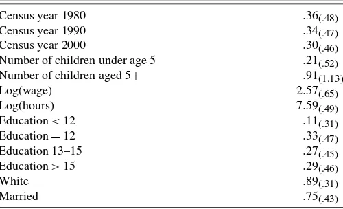
(16 birth years times 9 Census regions) and 432 (144 cohorts by 3 years) groups. As described in Section 2.1, the labor sup-ply equation is a log-linear hours–wage equation. The log of weekly hours in each group is a function of the log wage, in-dicator variables for the 144 cohorts, and inin-dicator variables for the 3 years. In addition, I include controls for marital status (a dummy that equals 1 if the individual is currently married and living with his spouse), number of children in the hold aged less than 5, and number of children in the house-hold aged 5 or older. The estimating sample is composed of 2,915,397 men. I carry out separate analyses by education level and by race. Descriptive statistics for the sample are given in Table 2.
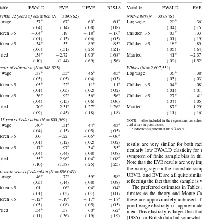
The estimated coefficients and standard errors by education group are given in Table 3. First, consider the EWALD results in the first column. These suggest a wage elasticity of about .4 for all four education groups. The presence of young children in the household leads to lower hours worked, with the effects being larger for the less educated groups. The presence of older children reduces hours for the lowest two education groups, but there is no evidence of this effect for the higher educated. In all four samples married men work significantly longer hours than other men. These results are all consistent with expectations.
The EVE results in the second column are much less pre-cisely estimated than their EWALD equivalents. For all but the lowest education group, the coefficient estimates are generally larger in absolute terms than EWALD, suggesting the EWALD bias is an attenuation bias for these samples. EVE seems partic-ularly problematic in the high school dropout sample in that the number of children coefficients and the married coefficient have
Table 2. Means of variables (standard deviations in parentheses)
Census year 1980 .36(.48)
Census year 1990 .34(.47) Census year 2000 .30(.46)
Number of children under age 5 .21(.52) Number of children aged 5+ .91(1.13)
Log(wage) 2.57(.65)
Log(hours) 7.59(.49)
Education<12 .11(.31)
Education=12 .33(.47)
Education 13–15 .27(.45)
Education>15 .29(.46)
White .89(.31)
Married .75(.43)
NOTE: The sample includes 2,915,397 observations.
284 Journal of Business & Economic Statistics, July 2007
Table 3. Labor supply estimates by education level
Variable EWALD EVE UEVE B2SLS
Less than 12 years of education(N=309,862)
Log wage .37∗ .67∗ .60∗ .61∗ (.04) (.14) (.08) (.08) Children>5 −.04∗ .19 −.18∗ −.16∗ (.01) (.13) (.06) (.05) Children<5 −.34∗ .53 −.89∗ −.85∗ (.06) (.51) (.25) (.21) Married .54∗ −2.72 1.90∗ 1.68∗ (.10) (1.44) (.69) (.56)
12 years of education(N=948,523)
Log wage .37∗ .55∗ .46∗ .45∗ (.03) (.05) (.04) (.03) Children>5 −.05∗ −.22∗ −.11∗ −.11∗
(.01) (.05) (.02) (.02) Children<5 −.36∗ −.92∗ −.56∗ −.56∗
(.04) (.15) (.06) (.06) Married .70∗ 2.31∗ 1.27∗ 1.26∗ (.09) (.45) (.18) (.18)
13–15 years of education(N=800,969)
Log wage .40∗ .31∗ .44∗ .43∗ (.04) (.15) (.05) (.05) Children>5 .00 −.22 −.05∗ −.06∗ (.01) (.12) (.02) (.02) Children<5 −.17∗ −.97∗ −.34∗ −.35∗ (.04) (.44) (.08) (.08) Married .55∗ 2.96∗ 1.04∗ 1.08∗ (.10) (1.38) (.25) (.25)
16 or more years of education(N=856,043)
Log wage .46∗ .72∗ .59∗ .58∗
(.05) (.14) (.08) (.08) Children>5 −.01 −.06∗ −.04∗ −.04∗
(.01) (.02) (.01) (.01) Children<5 −.12∗ −.19∗ −.17∗ −.17∗ (.03) (.08) (.05) (.05) Married .54∗ .57 .60∗ .62∗ (.11) (.36) (.19) (.19)
NOTE: Also included in the regressions are cohort dummies and year dummies. Stan-dard errors in parentheses.
∗indicates significant at the 5% level.
perverse signs. However, these coefficients are very imprecisely estimated.
The UEVE results in the third column are quantitatively quite different from both EWALD and EVE. The wage elasticity is uniformly higher than EWALD across education groups and is estimated to be about .6 for the high school dropouts and for college graduates, with values about .45 for the other groups. Likewise, the negative effects of children on labor supply (and the positive effects of marriage) are estimated to be larger us-ing UEVE than usus-ing EWALD, with the effects of both old and young children being negative and statistically significant for all four education groups. As expected, the UEVE results are less precisely estimated than EWALD but more precisely estimated than EVE. The B2SLS estimates and standard errors are gener-ally very close to UEVE, suggesting that heteroscedasticity is not a serious problem in this application.
In Table 4 I estimate the specification by race. Based on EWALD, one would conclude that the wage elasticity is signifi-cantly higher for whites than nonwhites. In contrast, the UEVE
Table 4. Labor supply estimates by race
Variable EWALD EVE UEVE B2SLS
Nonwhites(N=307,846)
Log wage .20∗ .36∗ .35∗ .37∗ (.04) (.15) (.07) (.07) Children>5 .03∗ .33 −.09 −.09
(.01) (.19) (.06) (.06) Children<5 −.18∗ .89 −.58∗ −.57∗ (.05) (.64) (.20) (.19) Married .41∗ −2.37 1.28∗ 1.24∗ (.09) (1.52) (.47) (.44)
Whites(N=2,607,551)
Log wage .36∗ .38∗ .37∗ .37∗ (.03) (.03) (.03) (.03) Children>5 −.04∗ −.08∗ −.06∗ −.06∗
(.01) (.01) (.01) (.01) Children<5 −.27∗ −.41∗ −.35∗ −.35∗
(.04) (.05) (.04) (.04) Married .87∗ 1.29∗ 1.10∗ 1.10∗ (.11) (.16) (.14) (.14)
NOTE: Also included in the regressions are cohort dummies and year dummies. Stan-dard errors in parentheses.
∗indicates significant at the 5% level.
results are very similar for both racial groups. Thus, the par-ticularly low EWALD elasticity for nonwhites appears to be a symptom of finite sample bias in this relatively small sample. Note that the EVE results are very imprecise and generally have the wrong sign in the nonwhite sample. In contrast, EWALD, UEVE, and EVE are all quite similar in the sample of whites, reflecting the fact that the sample is very large.
The preferred estimates in Tables 3 and 4 are the UEVE es-timates as the theory and Monte Carlo evidence suggest that these are approximately unbiased. These suggest an intertem-poral wage elasticity of approximately .4–.6 for all groups of men. This elasticity is larger than that found by Browning et al. (1985) for British data but somewhat smaller than the estimates of Angrist (1991) using U.S. data from the Panel Study of In-come Dynamics. The variation in the estimated elasticities and standard errors across estimators in Tables 3 and 4 implies that the choice of estimator may be of great importance in empirical practice.
One interesting feature of the application is that EWALD and UEVE are quite different despite the fact that the sample size is large relative to the number of groups. There are two fea-tures of the specification that help explain why finite sample issues are relevant to these seemingly large samples. The first is that there are four endogenous variables (wages, children aged less than 5, children aged 5 or older, and marital status) and the group means of these variables are correlated. The second is that both cohort and year fixed effects are included, and con-ditioning on these reduces the cross-group variance of wages substantially because the variance of wages over time within cohorts is much lower than the variance of wages across co-horts in the cross section.
Although reasonably small numbers of observations may be sufficient for precisely estimating group means, the presence of cohort and year fixed effects in cohort models increases enormously the likelihood of serious small sample biases in
EWALD and the number of observations required to eliminate biases. Thus, even if the variance of xg is low because there are many observations per group, it may still be sizable rela-tive to the cross-group variance inπg. Given the equivalence of EWALD to the 2SLS estimator using the microdata and group indicators as instruments, the finding here is similar to that of Bound et al. (1995) that 2SLS can be very biased in overi-dentified linear models even if the number of observations is very large. Devereux (2005) provided another example where EWALD suffers from small sample bias even with very large sample sizes.
6. CONCLUSIONS
This article has two main results. The first finding is that, with grouped data, EVE is identical to JIVE and, therefore, is biased in finite samples. Second, I show that one can use results from the instrumental variables literature to construct an unbiased EVE (UEVE) that is approximately unbiased in finite samples. Monte Carlo experiments support the theoreti-cal results and show that UEVE has both lower bias and vari-ance than EVE. In the intertemporal labor supply application, EWALD, EVE, and UEVE of the intertemporal wage elasticity are often quite different. This suggests that the choice of group-ing estimator is very relevant in practice.
Although UEVE is closely related to instrumental variables estimators, there are situations where the instrumental vari-ables estimators are infeasible but UEVE can be implemented using estimates of the group means and sampling variances. For example, Angrist (1990) used restricted Social Security Administration (SSA) data to examine the effects of Vietnam draft eligibility on earnings. For confidentiality reasons, the SSA would not provide individual-level data but did provide information on first and second moments of the variables by group. In this type of situation, UEVE could be implemented but conventional instrumental variables estimators are not fea-sible.
ACKNOWLEDGMENTS
I thank Dan Ackerberg, Joshua Angrist, Sandy Black, Janet Currie, Jin Hahn, Katerina Kyriazidou, Robert Moffitt, Donal O’Neill, Olive Sweetman, and Gautam Tripathi for helpful comments.
APPENDIX A: PROOF OF LEMMA 1
Following AIK, first I derive the bias ofβ=(X′C′X)−1× (X′C′Y) relative to the bias of β(Z), where β(Z) =
(′Z′X)−1(′Z′Y),
β−β(Z)
=(X′C′X)−1(X′C′Y)−β(Z)
=(′Z′X+η′C′X)−1(′Z′Y+η′C′Y)−β(Z). DefiningR=(′Z′X)−1, this can be written as
β−β(Z)
=R−1(I+Rη′C′X)−1(′Z′Y+η′C′Y)−β(Z) =(I+Rη′C′X)−1(R′Z′Y+Rη′C′Y)−β(Z).
Expanding(I+Rη′C′X)−1aroundRη′C′X=0 and ignoring terms of order less than 1/Ngives
β−β(Z)
=(I−Rη′C′X)(R′Z′Y+Rη′C′Y)−β(Z)+Op(1/N)
=R′Z′Y+Rη′C′Y−Rη′C′XR′Z′Y
−Rη′C′XRη′C′Y−(′Z′X)−1(′Z′Y)+Op(1/N)
=R′Z′Y+Rη′C′Y−Rη′C′XR′Z′Y −Rη′C′XRη′C′Y−R′Z′Y+Op(1/N)
=Rη′C′Y−Rη′C′Xβ(Z)−Rη′C′XRη′C′Y+Op(1/N)
=Rη′C′ε−Rη′C′X(β(Z)−β)−Rη′C′XRη′C′Y +Op(1/N).
The termRη′C′XRη′C′Yis of order lower than 1/N.
Expand-ing theith row ofX(β(Z)−β), one gets Xi(β(Z)−β)=Xi(′Z′X)−1(′Z′ε)
=Zi(′Z′Z)−1(′Z′ε)+Op(1/
√ N).
Then, expanding NR around R0 = plim(′Z′Z/N)−1 = (′z)−1, one can write
Rη′C′ε−Rη′C′X(β(Z)−β)
=N1(R0η′C′ε−R0η′C′PZε)+Op
1 N
,
where PZ = Z(′Z′Z)−1′Z′. E(β − β) = E(β −
β(Z))+E(β(Z)−β). The approximate bias ofβ(Z) equals−σεη(′z)−1/N. Hence,
E(β−β)=σεη(
′
z)−1 N E(C
′−C′P
Z−1)
=σεη(
′
z)−1
N trace(C−C
′P
Z−1).
Then, because CZ=Z, C′PZ=PZ. Also, because
trace(PZ)=K,
E(β−β)=σεη(
′z)−1
N
trace(C)−K−1. Note that if the homoscedasticity assumption is violated, trace(εη′C′PZ) now depends on the exact form of
het-eroscedasticity so the bias formula no longer has this simple form.
APPENDIX B: GROUP–ASYMPTOTIC PROPERTIES OF UEVE
B.1 Consistency of UEVE asG→ ∞
Deaton (1985) showed that EVE is consistent asG→ ∞. In this appendix I show the consistency of UEVE. Assume that
plim1 G
G
g=1
ngπgπ′g = ,
286 Journal of Business & Economic Statistics, July 2007
a positive-definite matrix. The probability limit of (1/G)× (Gg=1ngxgx′g−(G−K−1))asG→ ∞is as follows:
Together, (B.1) and (B.2) establish the consistency of the UEVE estimator asG→ ∞.
B.2 Group-Asymptotic Variance of UEVE
To simplify the notation, define
plim(Mxx)−α= ,
and the probability limits are taken as G→ ∞. Define the UEVE as
The exposition here closely follows Deaton (1985). Expanding (B.3) aroundβgives
β−β= −1[(Mxy−Mxxβ)−α(σ−β)]
−α −1[(σ−β )−(σ−β)] +Op(G−1). (B.5) The assumption of sampling under normality ensures that the second term is asymptotically independent of the first. Because the terms in (B.5) are sample averages centered around their means, by using a central limit theorem for independent but not identically distributed random variables one can show that √
G(β−β)is asymptotically normally distributed.
The asymptotic variance of β depends on the asymptotic variance of −1
Then, following Deaton, sampling under normality implies that the asymptotic variance ofσg−gβis
ngV{σg−gβ}
=(̺+β′β−2σ′β)+(σ−β)(σ−β)′. (B.7) Because(Mxy−Mxxβ) and(σ −β )are asymptotically independently distributed, the asymptotic variance–covariance matrix ofβis given by
To evaluate the variance–covariance matrix in practice requires estimates of and̺. These can be estimated as follows:
=Mxx−α,
̺=Myy−β′β.
Thus, the variance–covariance matrix can be estimated as
V{β} = 1 G
−1
[A+α2B]−1, (B.9) where
A=Mxx(Myy−β′β+β′β−2σ′β)
+(σ−β)(σ−β)′, (B.10)
B= 1 G
G
g=1
1 ng
(̺+β′β−2σ′β)
+(σ−β)(σ−β)′. (B.11) Note that the analogous variance–covariance matrices for EWALD, EVE, and the B2SLS estimator are calculated by evaluating (B.9) using values ofαequal to 0 for EWALD, 1 for EVE, and ((N−G)/(N−G+K+1))(G−K−1)/Gfor B2SLS.
[Received April 2004. Revised December 2005.]
REFERENCES
Acemoglu, D., and Pischke, J. S. (2001), “Changes in the Wage Structure, Family Income, and Children’s Education,”European Economic Review, 45, 890–904.
Ackerberg, D., and Devereux, P. (2003), “Improved Jive Estimators for Overi-dentified Linear Models With and Without Heteroskedasticity,” unpublished manuscript, University of California, Los Angeles.
Altonji, J. (1986), “Intertemporal Substitution in Labor Supply: Evidence From Micro Data,”Journal of Political Economy, 94, S176–S215.
Angrist, J. D. (1990), “Lifetime Earnings and the Vietnam Era Draft Lottery: Evidence From Social Security Administrative Records,”American Eco-nomic Review, 80, 313–336.
(1991), “Grouped Data Estimation and Testing in Simple Labor Supply Models,”Journal of Econometrics, 47, 243–265.
Angrist, J. D., Imbens, G. W., and Krueger, A. B. (1995), “Jackknife Instru-mental Variables Estimation,” technical report, National Bureau of Economic Research.
(1999), “Jackknife Instrumental Variables Estimation,”Journal of Ap-plied Econometrics, 14, 57–67.
Angrist, J. D., and Krueger, A. B. (1991), “Does Compulsory School Atten-dance Affect Schooling and Earnings?”Quarterly Journal of Economics, 106, 979–1014.
Bekker, P. A., and van der Ploeg, J. (1999), “Instrumental Variable Estimation Based on Grouped Data,” unpublished manuscript, Univeristy of Groningen.
Blomquist, S., and Dahlberg, M. (1994), “Small Sample Properties of Jackknife Instrumental Variables Estimators: Experiments With Weak Instruments,” unpublished manuscript, Uppsala University.
(1999), “Small Sample Properties of LIML and Jackknife IV Estima-tors: Experiments With Weak Instruments,”Journal of Applied Economet-rics, 14, 69–88.
Blundell, R., Duncan, A., and Meghir, C. (1998), “Estimating Labor Supply Responses Using Tax Reforms,”Econometrica, 66, 827–861.
Bound, J., Jaeger, D., and Baker, R. (1995), “Problems With Instrumental Vari-ables Estimation When the Correlation Between Instruments and the En-dogenous Explanatory Variable Is Weak,”Journal of the American Statistical Association, 90, 443–450.
Browning, M., Deaton, A., and Irish, M. (1985), “A Profitable Approach to La-bor Supply and Commodity Demands Over the Life-Cycle,”Econometrica, 53, 503–544.
Card, D., and Lemieux, T. (1996), “Wage Dispersion, Returns to Skill, and Black–White Wage Differentials,”Journal of Econometrics, 74, 319–361. Collado, M. D. (1997), “Estimating Dynamic Models From Time Series of
In-dependent Cross-Sections,”Journal of Econometrics, 82, 37–62.
Deaton, A. (1985), “Panel Data From a Time Series of Cross-Sections,”Journal of Econometrics, 30, 109–126.
Devereux, P. (2004), “Changes in Relative Wages and Family Labor Supply,”
Journal of Human Resources, 39, 696–722.
(2005), “Small Sample Bias in Synthetic Cohort Models of Labor Sup-ply,” unpublished manuscript, University of California, Los Angeles. Donald, S., and Newey, W. (2001), “Choosing the Number of Instruments,”
Econometrica, 69, 1161–1191.
MaCurdy, T. (1981), “An Empirical Model of Labor Supply in a Life-Cycle Setting,”Journal of Political Economy, 89, 1059–1085.
Mairesse, J., and Greenan, N. (1999), “Using Employee-Level Data in a Firm-Level Econometric Study,” in The Creation and Analysis of Employer– Employee Matched Data, eds. J. I. Lane, J. R. Spletzer, J. J. M. Theeuwes, and K. R. Troske, Amsterdam: Elsevier, pp. 489–514.
McClellan, M., and Staiger, D. (1999), “Estimating Treatment Effects Using Hospital-Level Variation in Treatment Intensity,” unpublished manuscript, Dartmouth College.
Mckenzie, D. J. (2001), “Consumption Growth in a Booming Economy: Tai-wan 1976–96,” unpublished manuscript, Economic Growth Center, Yale Uni-versity.
Nagar, A. L. (1959), “The Bias and Moment Matrix of the Generalk-Class Estimators of the Parameters in Simultaneous Equations,”Econometrica, 27, 575–595.
Neyman, J., and Scott, E. (1948), “Consistent Estimates Based on Partially Consistent Observations,”Econometrica, 16, 1–32.
Phillips, G. D. A., and Hale, C. (1977), “The Bias of Instrumental Variable Esti-mators of Simultaneous Equation Systems,”International Economic Review, 18, 219–228.
Ruggles, S., Sobek, M., Alexander, T., Fitch, C. A., Goeken, R., Hall, P. K., King, M., and Ronnander, C. (2004), Integrated Public Use Microdata Series: Version 3.0 [machine-readable database], Minneapolis: Minnesota Population Center [producer and distributor].
Staiger, D., and Stock, J. H. (1997), “Instrumental Variables Regression With Weak Instruments,”Econometrica, 65, 557–586.
Verbeek, M., and Nijman, T. (1993), “Minimum MSE Estimation of a Regres-sion Model With Fixed Effects From a Series of Cross-Sections,”Journal of Econometrics, 59, 125–136.