The Incredible Shrinking Elasticities
Married Female Labor Supply, 1978–2002
Bradley T. Heim
a b s t r a c t
This paper demonstrates the extent to which married women’s labor supply elasticities have changed over the past quarter century. Estimates from March Current Population Survey data suggest that these elasticities have decreased substantially, by 60 percent for the hours wage elasticity (from 0.36 to 0.14), 70 percent for the hours income elasticity (from -0.053 to -0.015), 95 percent for the participation wage elasticity (from 0.66 to 0.03), and 60 percent for the participation income elasticity (from -0.13 to -0.05). Changing demographic characteristics explain little of the drop in these elasticities, suggesting that preferences toward work have changed across birth cohorts.
I. Introduction
Estimates of labor supply elasticities are of key interest to policy-makers, since the responsiveness of labor supplies and labor force participation rates to changes in wages, incomes, and tax rates factor into the amount of revenue that tax increases raise and tax decreases will cost. In addition, the effectiveness of policies intended to encourage labor force participation and labor supply are in part deter-mined by these elasticities. Primarily due to research performed using data from the 1970s and 1980s, it is generally believed that married female labor supply elas-ticities are substantially larger than those of married men. This paper, however, dem-onstrates that female labor supply elasticities have dropped considerably over the past quarter century, both on the extensive and intensive margins.
Bradley Heim is a financial economist in the Office of Tax Analysis, U.S. Department of the Treasury. Substantial work on this paper was completed when the author was an Assistant Professor at Duke University. He wishes to thank Peter Arcidiacono, Marjorie McElroy, Bruce Meyer, Tom Mroz, Chris Taber, and Ron Warren, seminar participants at Duke University, the University of Wisconsin-Madison, the Federal Reserve Bank of Chicago, the University of Chicago Harris School, the 2005 SOLE Meetings and 2006 NTA Meetings, and two anonymous referees for helpful advice and comments. All remaining errors are the author’s. The views expressed are those of the author and do not necessarily reflect those of the Department of the Treasury. The data used in this article can be obtained beginning May 2008 through April 2011 from Bradley T. Heim, Office of Tax Analysis, U.S. Department of Treasury, Room 4036B, 1500 Pennsylvania Ave NW, Washington, DC 20220, or
Bradley.Heim@do.treas.gov.
[Submitted March 2006; accepted January 2007]
As has been documented numerous times, there exists a large literature focused on estimating male and female labor supply elasticities.1For men, these elasticities tend to be quite small,2 suggesting little responsiveness to changes in wages, nonlabor incomes, and tax rates. However, estimates of married women’s labor supply elastic-ities have tended to be substantially larger than men’s elasticelastic-ities. Killingsworth and Heckman (1986) surveyed the literature at the time and noted estimates of uncompen-sated wage elasticities ranging from -0.89 to 15.24, with a median of 0.76, and income elasticities ranging from -0.89 to 0.45, with a median of -0.09. More than a decade later, Blundell and MaCurdy (1999) surveyed the literature arising from methods that accounted for the piecewise linear shape of the budget constraint, and found uncom-pensated elasticities ranging from -0.01 to 2.03, with a median of 0.77, and income elasticities ranging from -0.40 to 0.52, with a median of -0.175. It is not surprising, then, that Killingsworth (1983) noted, ‘‘research indicates that structural responses (income and substitution effects) are considerably greater for women than for men,’’ a sentiment that was echoed a decade later by Heckman (1993).3
These high elasticities for married females imply that changes in income tax rates will have consequently greater effects. Further, responses to wage subsidy programs such as the Earned Income Tax Credit will be greater in absolute value. To the extent that these greater elasticities translate to greater compensated wage elasticities, the larger will be the deadweight loss from joint income taxation. In addition, sizable labor supply elasticity estimates are utilized in the specification of real business cycle models, and help to explain why hours worked vary more than does productivity.4
However, it is well documented that, over the past few decades, female labor force be-havior has undergone substantial changes, and labor force participation rates and annual hours of work among married women have increased markedly. Despite these dramatic increases, there has been little systematic attempt at examining whether the wage and in-come elasticities have changed as well. Indeed, Heckman (1993) noted, ‘‘whether labor supply behavior by sex will converge to equality as female labor-force participation con-tinues to increase is an open question.’’ Ten years later, this question remains open.
This paper, then, systematically examines the extent to which married women’s la-bor supply elasticities have decreased over the past quarter century. Using data from the Current Population Survey from 1979 to 2003, I show that both wage and income elasticities have dramatically declined, with more than a 60 percent decrease in the hours wage elasticity, more than a 70 percent decrease in the absolute value of the hours in-come elasticity, a 95 percent decrease in the participation wage elasticity, and more than a 60 percent decrease in the participation income elasticity. These findings are quite robust to the identifying variation, specification, and sample used.
1. See, for example, surveys in Hausman (1985), Pencavel (1986), Killingsworth and Heckman (1986), and Blundell and MaCurdy (1999), among many others.
2. See Hausman (1981), however, for a conflicting view, suggesting that men are more responsive to in-come taxation than others have suggested. See also MaCurdy et al. (1990), Eklof and Sacklen (2000), and Heim and Meyer (2004) who try to reconcile these two findings.
3. Heckman does note, however, that some estimates in Mroz (1987) come ‘‘fairly close to the low elas-ticities found for males by Thomas MaCurdy et al. (1990).’’
4. Kimmel and Kniesner (1998) note, for example, that ‘‘a relatively elastic labor supply is the core ele-ment of the labor market specification of empirical real business cycle models (Christiano and Eichenbaum 1992; Hansen and Wright 1992; Kydland 1995)’’
The estimated elasticities are then decomposed to examine the extent to which changes in the composition of married women, including their age distribution, ed-ucation, and childbearing patterns can explain this decrease. The results of this de-composition suggest that very little of the decrease can be explained by changes in the demographic composition of the married female labor force, suggesting that there have been substantial cross-cohort changes in preferences toward work. I sug-gest some possible explanations for these changes.
The paper proceeds as follow. Section II describes the data and the estimation strategy, and Section III summarizes some trends in the labor supply behavior of married women, as well as in their wages and incomes, that suggests that behavioral elasticities may have changed as well. Section IV presents the base results as well as the results from some robustness checks, and a comparison of these results to other findings in the literature. Section V probes whether changes in the demographic com-position of married females may explain why these elasticities have decreased. Sec-tion VI concludes.5
II. Data and Estimation Methodology
A. Sample Preparation
The 25 years of data used in this study come from the March Annual Demographic Survey of the Current Population Survey for the years 1979–2003. The Current Pop-ulation Survey (CPS) consists of short rotating panels, in which households are inter-viewed for four months, not interinter-viewed for the subsequent eight months, then interviewed an additional four months. They are then dropped from the sample. Interviews administered in the fourth and eighth months of the survey make up the Outgoing Rotation Group (ORG).
For the annual hours variable, the product of usual hours worked per week and weeks worked in the previous calendar year was used. Since the data reflect hours worked in 1978–2002, axes in the figures denote the years in which the hours were worked, and not the survey years.
For the hourly wage measure, one could divide each individual’s annual labor in-come by her annual hours of work. However, labor supply equations estimated using such a wage rate are well known to suffer from division bias, biasing wage elastic-ities downward.6Although this would be a concern in any labor supply study, in this study an additional concern arises, in that if errors in reported hours of work have increased (or decreased) over the past 25 years, estimates from these years would exhibit a downward (upward) trend, even absent any real trend in behavioral parameters.7
5. After completing the second draft of this paper, I became aware of a working paper by Blau and Kahn (2005) examining a similar topic. That paper looks at elasticities estimated at one decade intervals, does not examine robustness to the wage measure used, uses substantially different labor supply specifications, and does not exam-ine whether demographic characteristics can explain the decrease in estimated elasticities. However, the fact that their paper comes to a similar conclusion suggests that the finding in this paper is quite robust.
6. See, for example, Eklof and Sacklen (2000).
7. However, as a robustness check, the base specification is also run using the full sample and the labor income divided by hours wage measure.
Therefore, for the hourly wage variable, this study utilizes a series of questions, added in 1979 for those in the ORG of the CPS, which ask for information on each individual’s typical hourly or weekly wage.8 Because this wage measure is only available beginning in 1979, it is then that the time frame of analysis begins. In ad-dition, since this wage measure can only be created for members of the ORG, the sample was cut to include only those who were members of the ORG at the time of the March survey for most of the specifications in this paper.9
To construct this wage variable, the following algorithm was used. If the respon-dent reported an hourly wage, this variable was used. If they reported their wage as an amount that they received each week, that amount was divided by their usual hours per week, or by 40 if they did not report a usual hours per week.10Although the directly reported hourly wage eliminates the possibility of division bias, the wage measure derived from weekly earnings may still embody some division bias. How-ever, such a bias should be less in magnitude than the bias that arises when using the annual income divided by annual hours measure of wages, since there are two sour-ces of error in that measure (error in usual hours worked per week, and error in weeks worked per year).11
The nonlabor income variable was created by adding the asset income of the cou-ple to the labor income of the husband, and so a secondary earner model of labor supply is implicitly assumed.
Finally, in addition to those listed above, several other variables were utilized, in-cluding the wife’s age, education, race, number of children, the presence of children younger than six, geographic variables, and the unemployment rate in the wife’s
8. This wage variable is still not perfect, however, since some recent research (see, for example, Lemieux 2006) has documented that measurement error in the CPS ORG has gotten worse over time, which could result in a downward trend in estimated elasticities due to attenuation bias. Two factors ameliorate this concern, how-ever. First, instrumental variables are used in all specifications, and to the extent that these instruments are uncorrelated with the error in the wage variable, the resulting estimates will be purged of attenuation bias. Sec-ond, when identification comes solely from variation in tax rates in a robustness check, the declines from the base specification are still apparent, suggesting that attenuation bias alone is not driving the results. 9. Unfortunately, due to some peculiarities in the sampling frame of the March CPS in some years, not all individuals who were in the ORG received the hourly or monthly earnings questions, and these individuals are not identified in any particular way in the data set. The major cause of this in recent years is the increase in the March sample used to evaluate the SCHIP program, but several other reasons exist for other years. This is a problem for those who are nonworkers, as it is impossible to tell whether or not a nonworker was part of the ORG who would have received the earnings questions had they worked. As a result, if you cut only those who were working and had a nonresponse to the ORG questions, the labor force participation rate for the resulting sample is much below the labor force participation rate of the overall sample. As such, the sample includes all those with positive hours who have a valid response to the hourly earnings questions, and a random sample of nonworkers, so that the labor force participation rate in the resulting sample equals the labor force participation rate in the overall sample.
10. For variables that are topcoded, the algorithm in Lemieux (2006) was followed for imputing wages. For 1985 forward, the topcoded hourly earnings value was multiplied by a factor of 1.4 to yield the hourly wage. For topcoded weekly earnings, the topcoded value was multiplied by a factor of 1.4, then divided by usual weekly hours to yield the wage. For annual earnings before 1989, the topcoded value was multi-plied by 1.4, then divided by annual hours of work. For 1989-95, annual income was re-topcoded to $99,999, and annual income for 1998-2003 is re-topcoded to $150,000, for consistency. These re-topcoded values are then multiplied by 1.4, and divided by annual hours to yield the wage.
11. Although this wage measure has the advantage that it does not suffer from division bias, it does not include income from second jobs or overtime work.
state. All monetary variables were inflated or deflated to real dollars from the year 2000, using the CPI-Urban Price Index.
The sample includes married women who are between the ages of 25 and 55 in order to focus on labor supply behavior in the prime working years. Those who are self-employed, students, retired, or disabled were excluded, as well as those for whom either wage measure cannot be created due to nonresponse. In addition, individuals who reported working an extreme number of hours, over 4,200 hours an-nually, were excluded.12Sample statistics for all variables among those who were in the ORG are presented, by year, in an appendix available online, associated with the abstract of this article, at www.ssc.wisc.edu/jhr/.13
B. Estimation Method
For this study, the ideal practice would be to use a generally agreed-upon standard estimation method to estimate married female labor supply. However, such a meth-odology does not exist.
Indeed, in recent years, several methodologies have been proposed. For example, Blundell et al. (1998) use difference in differences techniques and tax reforms to es-timate labor supply elasticities, utilizing variation in tax rates across individuals and across time. Some recent papers have used difference in differences or reduced form methodologies to identify labor supply parameters, including Kimmel and Kniesner (1998), Eissa (2001), Eissa and Hoynes (2004, 2006), and others. Several other recent papers, among them van Soest (1995), Hoynes (1996), and Heim (2006), es-timate structural models of the joint labor supply choices of a husband and wife. These studies tend to assume that wage rates are exogenous, and use variation in wages and incomes across individuals, as well as tax rates in some cases, to identify labor supply elasticities.
In addition, if one goes further back in the literature to studies surveyed in Killingsworth (1983), one finds studies that use variation in wages and labor supply by demographic group to identify labor supply estimates, utilizing exclusion restric-tions on how age and education affect labor supply.
Utilizing any of these methods directly and in isolation for this study is problem-atic. The older studies have been criticized for using instruments that are likely in-valid to estimate labor supply elasticities. To estimate elasticities separately for each year using difference in differences, one would need policy changes every year that either affected all married women (to get an overall elasticity estimate) or policy changes that affected the same group every time (to get a subsample specific esti-mate). However, such policy changes simply do not exist, and if one used the policy changes that did occur, the elasticity estimates would likely differ because the esti-mates are identified from different subsets of women. Finally, the structural methods are simply too computationally intensive to estimate separate parameters for each of 25 years of data.
12. Sample sizes, by year, after the various sample cuts, are presented in an appendix available online, as-sociated with the abstract of this article, at www.ssc.wisc.edu/jhr/.
13. Sample statistics, by year, for the full March CPS sample are presented in an appendix available online, associated with the abstract of this article, at www.ssc.wisc.edu/jhr.
Thus, in an attempt to keep the estimates in this study roughly comparable to others in the literature, this study uses similar sources of variation to each of these methodologies to identify labor supply elasticities, while still maintaining a specifi-cation that can be estimated on each year of data. To do so, this study uses an adap-tation of the ‘‘second generation’’ methods reviewed in Killingsworth (1983), or the selection-corrected methodology described in Mroz (1987), with an extra step added to estimate extensive margin elasticities.
Estimation proceeds in four stages. In the following, coefficients are subscripted witht
to emphasize that separate systems of equations were estimated for each year of data. In the first stage, a reduced form probit of the form
Pit=a0t+a1tYit+a2tZPit+e
is run, wherePit= 1 denotes participation,Yitdenotes nonlabor income, andZitP con-tains other variables that affect the participation decision. Included inZitPare a cubic in age and years of education, race dummies, the number of children, the presence of children younger than six, the unemployment rate in the state of residence, and geo-graphic variables including a regional dummy, a dummy for residence in a center city, and the size of the MSA of residence.
In the second stage, a selection corrected wage regression of the form
lnWit =b0t+b1tZitW+e W it
ð2Þ
is run on those observed working positive hours who have a wage report. Included in
ZW
itare a cubic in age and years of education variables, race dummies, the geographic variables noted above, and the inverse Mills ratio calculated from the first stage. The method up to this point is simply the Heckman two-step method, described in Heckman (1980). The exclusion of nonlabor income and children variables in this equation provides identification of the inverse Mills ratio term other than that which would come from functional form assumptions alone.
In the third stage, a selection corrected labor supply equation of the form
hit=g0t+g1tlnWˆit+g2tYit+g3tZhit+e h it
ð3Þ
is estimated on women observed working positive hours, where lnWˆit denotes the wage imputed from the second stage.14Regressors other than the wage and
non-labor income variables in this equation include the woman’s age, years of education, number of children, the presence of children younger than six, unemployment and geographic variables, and the inverse Mills ratio calculated from the first stage.15
14. Specifications linear in the wage variable were also run. The results were qualitatively similar to those presented here.
15. Note that, in this specification, the identification of the inverse Mills ratio comes from functional form assumptions. In a specification check, geographic variables are excluded from the hours equation, aiding in identification of the inverse Mills ratio. These results are presented in an appendix available online, asso-ciated with the abstract of this article, at www.ssc.wisc.edu/jhr. The results are qualitatively similar for the hours income elasticity and participation elasticities, but the hours wage elasticity does not exhibit a decline in this specification.
Identification of the wage coefficient comes from the exclusion of higher order terms in age and education. Using the estimates from this stage, hours elasticities were cal-culated as
where ˆg1t and ˆg2t denote the estimated coefficients on log wages and nonlabor in-come, respectively,ht denotes mean annual hours of work conditional on working, andYtdenotes mean nonlabor income.
As robustness checks, the elasticities were reestimated using several other speci-fications, including a specification in which taxes are accounted for in a simple man-ner to aid in identification of the elasticities, a specification in which wages are assumed to be exogenous, and a specification in which the full CPS sample was used and the wage variable was created by dividing labor income by annual hours.16
In the fourth stage, a structural participation equation of the form
Pit=d0t+d1tlnWˆit+d2tYit+d3tZitP+e
is estimated. Identification of this equation follows the same strategy as described above for the hours equation, and most of the robustness checks described above were performed. Participation elasticities were calculated as
ep
@lnW denotes the estimated average derivative of participation with respect to log wages, and@ˆF
@Y denotes the estimated average derivative with respect to nonlabor income.
Implicit in this estimation method is the assumption that the wife chooses her hours of work conditional on her husband’s choices, and so there is no joint utility maximi-zation or bargaining occurring in this model. Further, exogeneity of marital status and of childbearing is assumed. Although a more complex structural model of the choice of marriage, childbearing, and labor force behavior that incorporates interactions
16. In an appendix available online, associated with the abstract of this article, at www.ssc.wisc.edu/jhr, several other specifications were estimated, including a specification in which geographical variables are excluded from this step to align the specification more closely with Mroz (1987), a specification in which all age and education interactions are included in this step so that identification comes solely from variation in tax rates, an adaptation of the life cycle consistent model in Ziliak and Kniesner (1999) to examine the robustness to a nonstatic model, and a specification in which the inverse Mills ratio is omitted to examine the robustness to not accounting for sample selection.
between the husband and wife may yield additional insights into the source of the trends found here, such an undertaking is beyond the scope of this paper.
Standard errors of the estimated elasticities were bootstrapped, to account for the multistage nature of the estimation method. In addition, all regressions were per-formed using the weights provided in the CPS, due to the changes in the sampling frame in the 2002 and 2003 March CPS.
III. Labor Supply, Wage, and Income Trends
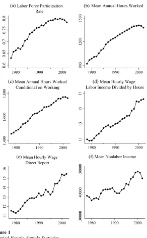
To provide some context for the results that follow, this section pres-ents the time path of some variables from the sample used in this study. In Figure 1, labor force participation rates, mean unconditional hours of work and hours of work conditional on working, mean wages, and mean incomes are presented for all of the years under study.
In Panel A of this figure, the married female labor force participation rate has in-creased from slightly more than 63 percent to 79 percent in the past 25 years. As a basis of comparison, Blundell and MaCurdy (1999) note that overall female labor force participation increased from just less than 50 percent to slightly more than 60 percent from the years 1979 to 1994. Hence, married women aged 25 to 55 tend to have higher labor force participation rates than women as a whole, but the rate of increase in labor force participation has been just as dramatic despite the higher start-ing point.
In Panel B, mean annual unconditional hours of work also exhibits an upward trend, increasing from 915 hours in 1978 up to more than 1,350 in 2002, an increase of almost 50 percent. This increase is not only due to married women entering the labor force. In Panel C, mean annual hours of work conditional on working some hours in the year are presented, and these also have increased, from 1,450 hours in 1978 to more than 1,750 hours in 2002.
Turning to wages, Panel D presents the trend in mean real hourly wages among married women who are working, when the wage is calculated by dividing labor in-come by hours worked, while Panel E contains the time trend in mean real hourly wages when the direct report of the wage is used.17Both of these figures demonstrate a substantial increase in wages over this time period, from around $11/hour (in 2000 dollars) in 1978 up to more than $15/hour (in 2000 dollars) in 2002.
Finally, in Panel F mean nonlabor income for all women is presented, where non-labor income is defined as asset income plus the non-labor income of the husband. Al-though the increase in nonlabor income is not as dramatic as the increase in wages displayed above, there still appears to be an upward trend in nonlabor income, particularly since 1992.
Thus, measures of labor force participation, hours, wages, and nonlabor income have all increased substantially for married prime-age females. It is plausible that, along with these trends, there was a change in the overall responsiveness of the
17. This figure contains wages that are reported in the ORG earners’ study, including both reported hourly wages and wages that are calculated by dividing weekly wages by weekly hours.
Figure 1
Married Female Sample Statistics
various dimensions of labor supply to wages and income, and so it is to this issue that this paper turns next.
IV. Overall Trends in Elasticities
In the figures that follow, estimated wage and income elasticities, both on the extensive and intensive margin, are presented. These figures suggest that both wage and income elasticities along both the extensive and intensive margins have decreased by large magnitudes over the past two and a half decades. These decreases are primarily driven by decreases in estimated coefficients and not by increases in mean annual hours worked or labor force participation rates that enter into the denominator of the elasticity. Further, these results are largely robust to the identifying variation, sample, and wage variable used in the estimation specification.
A. Base Specification
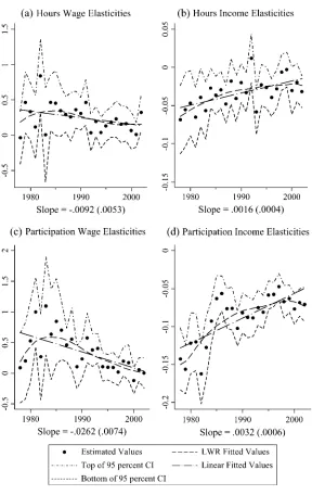
In Figure 2, the estimated elasticities from the base specification are presented. In each panel of the figure, the estimated elasticities are plotted along with the top and bottom of the 95 percent confidence interval of the estimated elasticity, so that the significance of individual estimates and changes across estimates can be gauged. In addition, the fitted values from both a linear and a locally weighted regression18of the elasticity estimates against a time trend are presented, so that any trend can be discerned when one abstracts away from the noise in individual years’ estimates. Fi-nally, the slope of the linear time trend (and its standard error) is presented, so that it is possible to decipher the implied magnitude and significance of the yearly decline in each of these elasticities. The coefficient estimates that correspond to the elastic-ities in this figure are presented in Table 1.
Estimated hours wage elasticities are presented in Panel A of Figure 2. The esti-mates in this figure display a slight downward trend, despite the large standard errors on the estimates, and the results from the linear regression bear this out. The slope of this regression line is -0.0092 with a standard error of 0.0053. The fitted values hover around 0.35 in 1980, but drop to approximately 0.22 by the end of the sample. Due to a small negative estimated elasticity for 1978, the locally weighted regression fol-lows a hump-shaped pattern, but abstracting away from this outlier, estimated hours elasticities appear to have fallen by 61 percent over the 25 years in the sample.
Estimated hours income elasticities are presented in Panel B, in which the esti-mated elasticities trend up toward zero. The linear regression line has a slope of 0.0016 with a standard error of 0.0004, implying an increase of more than 0.038 over the sample period, a decrease in magnitude of more than 70 percent. Further, the fit-ted values from the locally weighfit-ted regression follow the linear trend line quite closely, though it does appear to level off toward the end of the period.
In Panels C and D of Figure 2, participation wage and income elasticities are pre-sented. In Panel C, the linear trend line suggests that participation wage elasticities have decreased from 0.66 to 0.03 (with the slope of the linear regression being
18. See Cleveland (1979).
Figure 2
Estimated Wage and Income Elasticities
-0.0262 with a standard error of 0.0038), although low estimated elasticities in 1978 and 1979 give the nonlinear trend a hump shape with elasticities peaking in the early 1980s before declining to close to 0 by the end of the sample. Income elasticities in Panel D increase toward 0 from -0.128 to -0.049 (with the slope of the linear regres-sion being 0.0032 with a standard error of 0.0006), implying a decrease of more than 60 percent.
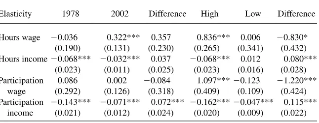
These results are further summarized in Table 2, which presents the difference in elasticities from the beginning to end of the period, as well as the difference between the high- and low-estimated elasticity over this time period.
For the 1978-2002 differences, the only significant difference is for the participa-tion income elasticity. However, for the hours income and participaparticipa-tion wage elastic-ities, the magnitudes of the differences are quite large. For example, the hours income elasticity estimated in 2002 is less than half the size of the estimate from 1978 and the participation wage elasticity from 2002 is less than 5 percent of the size of the estimate from 1978. The hours wage elasticity increases between 1978 and 2002, but the estimated difference is insignificant, and the increase is largely due to the estimated elasticity from 1978 being substantially below the estimates from subsequent years, and the estimate from 2002 being substantially above the estimates from preceding years.
Nevertheless, all high-low elasticity differences in this table are significant. In ad-dition, the high elasticity estimates all come from years prior to the low estimates, and the differences in these elasticities suggest large drops in elasticities between the high and low years.
As a specification check, Table 1 presents results from tests for weak instruments, by year, including the partialR-squared of the instruments in the first stage equation, and theFtest statistic and the related p-value from a test that the coefficients on all instruments are zero. As noted in Staiger and Stock (1997),Ftest statistics above 10 are preferable to avoid weak instrument concerns, but unfortunately only in one year is theFtest statistic above 10 for the ORG sample used here. Two factors, however, ameliorate this concern. First, as can be seen in Appendix Table A1, when the entire sample is used in a robustness check theFtest statistic is substantially above 10 in most years, even though the partialR-squareds tend to be lower than for the ORG sam-ple. Second, when several robustness checks are performed below including accounting for taxes to aid in identification and not instrumenting for the wage, the results are qualitatively similar, suggesting that the strength of the instruments is not driving the general result that there have been substantial declines in these elasticities. It is possible, however, that the elasticities in Figure 2 decline not because the changes in the estimated coefficients, but instead because of changes in means of the variables that are used in calculating the elasticities, particularly because of increases in labor force participation rates and hours of work, which enter into the denominator of the elasticities. Were this the case, it would be hard to attribute the change in elasticities to a change in labor supply preferences, because a given percentage increase in income or wages would lead to the same change in number of hours or labor force participation rates. On the other hand, increasing wage and income levels would tend to dampen any decrease in estimated elasticities.
Table 1
Estimation Results and Specification Test Statistics Outgoing Rotation Group Sample
1978 1979 1980 1981 1982 1983 1984
Estimated coefficients - hours equation
Wage 256.8 747.0 533.7 189.2 1374.5 10.4 768.6
(301.7) (357.0) (331.2) (376.0) (435.9) (560.5) (337.2)
Nonlabor income 20.0028 20.0024 20.0020 20.0029 20.0017 20.0025 20.0012
(0.0009) (0.0010) (0.0009) (0.0009) (0.0009) (0.0008) (0.0006)
Estimated average derivatives - participation equation
Wage 0.051 0.121 0.317 0.611 0.166 0.688 0.427
(0.172) (0.195) (0.203) (0.177) (0.223) (0.257) (0.254)
Nonlabor income 22.18E-6 22.52E-6 21.98E-6 21.98E-6 22.71E-6 22.15E-6 21.59E-6
(3.16E-7) (2.62E-7) (3.31E-7) (3.17E-7) (3.32E-7) (3.49E-7) (2.47E-7)
First Stage Test Statistic
Partial R2 0.0121 0.0074 0.0049 0.0043 0.0037 0.0042 0.0028
Ftest 5.1 3.61 2.39 1.96 1.72 1.92 1.38
p-value 0.000 0.001 0.019 0.056 0.099 0.063 0.209
1985 1986 1987 1988 1989 1990 1991
Estimated coefficients - hours equation
Wage 767.8 579.4 500.1 442.7 621.7 534.0 811.6
(395.5) (309.1) (217.3) (299.2) (230.7) (204.6) (288.9)
Nonlabor income 20.0015 20.0012 20.0020 20.0008 20.0017 20.0009 20.0015
(0.0005) (0.0005) (0.0005) (0.0006) (0.0006) (0.0006) (0.0006)
(continued)
Heim
Table 1 (continued)
1985 1986 1987 1988 1989 1990 1991
Estimated average derivatives - participation equation
Wage 0.564 0.505 0.340 0.400 0.077 0.172 0.439
(0.238) (0.176) (0.103) (0.188) (0.135) (0.123) (0.159)
Nonlabor income 21.04E-6 29.82E-7 21.39E-6 21.36E-6 21.86E-6 21.51E-6 21.72E-6
(2.54E-7) (2.05E-7) (2.43E-7) (2.59E-7) (2.11E-7) (2.45E-7) (2.68E-7)
First stage test statistic
Partial R2 0.0029 0.0021 0.0072 0.0078 0.0035 0.0087 0.0097
Ftest 1.47 1.11 3.59 4.42 2.13 5.3 6.29
p-value 0.171 0.353 0.001 0.000 0.037 0.000 0.000
1992 1993 1994 1995 1996 1997 1998
Estimated coefficients - hours equation
Wage 63.5 343.9 64.0 231.9 332.2 416.2 285.4
(236.1) (192.0) (194.9) (199.4) (194.3) (237.8) (243.7)
Nonlabor income 0.0005 20.0025 20.0010 20.0011 20.0017 20.0011 20.0003
(0.0007) (0.0006) (0.0006) (0.0006) (0.0005) (0.0005) (0.0005)
Estimated average derivatives - participation equation
Wage 0.292 0.320 0.081 0.077 0.074 0.014 0.154
(0.106) (0.098) (0.094) (0.085) (0.102) (0.089) (0.095)
Nonlabor income 21.71E-6 21.43E-6 21.55E-6 21.08E-6 21.09E-6 28.34E-7 21.18E-6
(2.35E-7) (2.26E-7) (2.15E-7) (1.76E-7) (1.51E-7) (1.57E-7) (1.93E-7)
(continued)
894
The
Journal
of
Human
Table 1 (continued)
1992 1993 1994 1995 1996 1997 1998
First stage test statistic
Partial R2 0.0148 0.0071 0.0182 0.0135 0.0138 0.0039 0.0093
Ftest 9.56 4.04 10.74 6.93 7.06 1.98 4.88
p-value 0.000 0.000 0.000 0.000 0.000 0.054 0.000
1999 2000 2001 2002
Estimated coefficients - hours equation
Wage 303.7 123.6 14.9 597.2
(232.5) (246.6) (165.7) (242.6)
Nonlabor income 20.0001 20.0012 20.0008 20.0013
(0.0004) (0.0006) (0.0005) (0.0004)
Estimated average derivatives - participation equation
Wage 0.137 20.099 0.044 0.002
(0.120) (0.087) (0.078) (0.100)
Nonlabor income 21.05E-6 21.26E-6 21.14E-6 21.19E-6
(1.50E-7) (1.67E-7) (1.51E-7) (1.97E-7)
First stage test statistic
Partial R2 0.0054 0.0105 0.0081 0.0071
Ftest 2.69 5.14 5.46 4.71
p-value 0.009 0.000 0.000 0.000
Note: Bootstrapped standard errors are in parentheses. Heim
participation rate variables over all years. Because all variables are now held at their mean values across all years, any movement in elasticities in these graphs is due solely to movement in the estimated coefficients. Comparing this figure to Figure 2, the decline in estimated elasticities is similar to what it was in that figure, suggest-ing that changsuggest-ing means of variables are not the primary cause of the decline in elasticities.
One might still worry, however, that the changing labor force participation rate is affecting the estimated participation elasticities through the calculation of the aver-age derivative. The averaver-age derivative is calculated by multiplying the estimated co-efficient from the probit by the density of the standard normal pdf at the mean of righthand side variables in Equation 4 (call these theXb0s). If theX’shave increased so that more individuals are participating in the labor force, this would result in the density of the standard normal being evaluated further toward the tail, thus decreas-ing its magnitude. As a result, the estimated elasticities could decrease even with no change in estimated coefficients.
To examine whether this is the case, Figure 4 presents the estimated probit coef-ficients from each year, as well as the standard normal pdf at the mean of theXb0s, denoted asfðXbÞ. In this figure, it is clear that, although a decreasing trend infðXbÞ
contributes to decreases in the elasticities, decreases in estimated coefficients play a role as well.
Taken together, these figures suggest that changing values of mean annual hours and labor force participation variables are not driving the changes in estimated elasticities.
B. Accounting for Taxes
One possible concern with the specification used above is that it does not incorporate taxes. Accounting for taxes is desirable for three reasons. First, since wage and in-come elasticities are often used to simulate the effects of changes in tax rates, a Table 2
Results from Base Specification Difference in Estimated Elasticities
Elasticity 1978 2002 Difference High Low Difference
Hours wage 20.036 0.322*** 0.357 0.836*** 0.006 20.830*
(0.190) (0.131) (0.230) (0.265) (0.341) (0.432) Hours income20.068*** 20.032*** 0.037 20.068*** 0.012 0.080***
(0.023) (0.011) (0.025) (0.023) (0.016) (0.028) Participation
Note: Bootstrapped standard errors are in parentheses.
Figure 3
Estimated Wage and Income Elasticities Evaluated at Mean of All Variables
Figure 4
Decomposition of Average Derivatives
specification that controls for taxes would be preferable. Second, variation in tax rates and amounts across individuals aids in the identification of wage and income coefficients. Third, if taxes aren’t accounted for, the estimates above may be biased, and if the bias exhibits a trend over the period, declining elasticities could result due to a model misspecification.
For these reasons, and as a specification check, the specification above was mod-ified to account in a simple way for taxes, without having to resort to a structural estimation method that explicitly models the entire shape of the budget constraint.
To do so, the NBER’s TAXSIM model was used to calculate the marginal tax rate and taxes owed for each woman in each year at 0 hours of work and at 2000 hours per year. To calculate the tax variables, each woman’s actual nonlabor income was used, but for labor incomes the state specific mean of husbands’ and wives’ labor incomes were used (including nonworkers) in order to eliminate the endogeneity of the tax rate to the woman’s own labor supply and wages and her spouse’s labor supply.19 For these calculations, it is assumed that everyone takes the standard deduction, and that they claim a number of dependents equal to the number of children younger than 18 within the household. The calculated marginal tax rates and taxes owed used in the estimation include both federal and state income taxes, the employee’s share of the payroll tax, and federal and state Earned Income Tax Credits.
Using these calculated tax variables, the estimation method outlined above was al-tered as follows. In the reduced form participation probit, the log of the net of tax share at 0 hours of work, lnð12t0itÞ, was added as a regressor, and gross nonlabor income was replaced with nonlabor income net of taxes at 0 hours of work. In the selection corrected labor supply equation, the predicted log wage and gross nonlabor income were replaced with the log of the predicted wage multiplied by the marginal tax rate at 2000 hours of work, lnðð12t2000ÞWÞˆ , and the virtual income associated
with that budget segment.20Finally, in the structural probit equation, the log wage and gross nonlabor income were replaced with the log of the predicted wage multi-plied by the marginal tax rate at 0 hours of work, lnðð12t0ÞWÞˆ , and nonlabor income net of taxes at 0 hours of work.21
Variation in the tax variables exists at the state level, due to different state spe-cific labor income variables, and at the individual level, because of different num-bers of dependents and amounts of nonlabor income. Across years there exists substantial variation in these marginal tax and taxes owed variables.
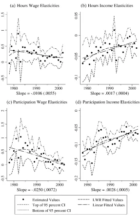
Figure 5 presents the results from this specification.22Comparing this figure to Figure 2, the results above are remarkably robust to this specification change. All
19. If this endogenous tax rate were to be used in the specification, one would then have to instrument for the tax rate, requiring further exclusion restrictions, most of which are implausible. (See Heim and Meyer (2004)).
20. For a discussion of virtual income, see MaCurdy (1992).
21. This step is similar to the method used in Eissa and Hoynes (2004), with the average full time tax rate in their specification replaced with the marginal rate at 0 hours used here.
22. An alternative method would be to use the actual log net of tax wage in the second stage wage regres-sion, instrumenting for the endogenous tax rate, and then use predicted net of tax wages in Stages 3 and 4. However, experimentation with such a method resulted in implausible large negative participation wage elasticities, and so that approach was rejected in favor of the one used here.
elasticities decrease over the time period under analysis, and the magnitudes are sim-ilar to those in the base specification, with the linear trend lines exhibiting a 50 per-cent decline in the hours wage elasticity (from 0.2 to 0.1), a 75 perper-cent decline in the hours income elasticity (from -0.045 to -0.01), a 100 percent decline in the partici-pation wage elasticity (from 0.5 to 0), and a 60 percent decline in the participartici-pation income elasticity (from -0.115 to -0.045).
To examine the robustness of these results to the specification of taxes, specifica-tions were also estimated in which tax variables at 0 hours were used through all steps, and in which tax variables at 2,000 were used. In addition, a specification was estimated in which interactions between age and education were included in the structural labor supply and participation equations, so that the wage elasticities are identified solely from variation in tax rates. Those results are generally similar to those presented here, and are available in an online appendix, associated with the abstract of this article, at www.ssc.wisc.edu/jhr/.
C. Assuming Wages are Exogenous
All of the specifications above assumed that gross wages are endogenous. However, in some work, particularly structural work, it is typically assumed that wages are exogenous.23
To examine whether these elasticities have declined if one makes the assumption that wages are exogenous, a reduced-form participation probit was run, followed by a selection corrected labor supply regression on all workers in the sample, using the uninstrumented gross wage as a regressor. Under such a procedure, the structural par-ticipation probit cannot be used to calculate parpar-ticipation elasticities, since wages are not observed for nonworkers. Thus, only the hours wage and income elasticities are presented.
Figure 6 presents the results from this specification. The hours wage elasticity decreases from 0.24 to 0.12 and the hours income elasticity decreases from -0.06 to -0.03, decreases of one-half. Thus, the results presented above are robust to assum-ing that wages are exogenous, in that both the magnitudes of the estimates and the magnitudes of the decreases in them are similar to the base specification.
D. Full Sample with Alternative Wage Measure
Finally, to examine whether the results presented above are robust to using an alter-native wage measures, the base specification was rerun using the full CPS sample and a wage created by dividing annual labor income by annual hours. Figure 7 pres-ents these results.
In this specification, most of the results found above hold, with the exception that the hours wage elasticity now displays a minuscule downward trend. Most likely, this is driven by two forces working in opposite directions. In early years, the true elas-ticity is high, but division bias results in a lower estimated elaselas-ticity. As the years
Figure 5
Estimated Wage and Income Elasticities: Accounting for Taxes
progress, the true elasticity decreases, but due to improvements in the Current Pop-ulation Survey, measurement error in hours decreases, resulting in division bias being less of a factor. As a result, there exists a smaller drop in the estimated elas-ticities than there would have been without this change in the magnitude of division bias.
Overall, then, it appears that the results presented above are not an artifact of the wage measure that was used in the base specification.
E. Other Robustness Checks
Several other specifications were also estimated, including a specification in which geographical variables are excluded from the selection corrected labor supply equa-tion to align the specificaequa-tion more closely with Mroz (1987), a specificaequa-tion in which all age and education interactions are included in the structural labor supply and labor force participation equations so that identification comes solely from var-iation in tax rates, an adaptation of the life cycle consistent model in Ziliak and Kniesner (1999) to examine the robustness to a nonstatic model, and a specification in which the inverse Mills ratio is omitted to examine the robustness to not account-ing for sample selection.
Figure 6
Estimated Wage and Income Elasticities: Wage Assumed Exogenous
Figure 7
Estimated Wage and Income Elasticities: Full Sample Using Alternative Wage Measure
In general, the results were qualitatively similar to those presented here, with two exceptions: the hours wage elasticity did not exhibit a decline when geographic var-iables were excluded, and the participation wage elasticity did not exhibit a decline when a life cycle consistent model was estimated. Results from all of these specifi-cations are presented in an appendix available online, associated with the abstract of this article, at ww.ssc.wisc.edu/jhr/.
F. Reconciliation with Other Results in the Literature
In the base estimation specification, hours wage elasticities were estimated to have decreased from 0.36 to 0.14, hours income elasticities fell from -0.053 to -0.015, par-ticipation wage elasticities fell from 0.66 to 0.03, and parpar-ticipation income elastici-ties fell from -0.13 to -0.05. In a recent working paper, Blau and Kahn (2005) also examine married female labor supply elasticities over time by looking at three groups of March CPS data, from 1979-81, 1989-91, and 1999-2001. They find, in their base specification, decreases in the hours wage elasticity from 0.8 - 0.9 in the earliest pe-riod down to 0.4 in the latter pepe-riod. Thus, although the estimated drop in percentage terms is similar to that found here, the magnitude of the elasticities throughout the period are substantially larger than those found here.
Two aspects of this specification, however, are likely causes for this discrepancy. First, these estimates come from a basic linear IV regression in which nonworkers are included as having zero hours of work, and so these estimates confound responses on the extensive and intensive margins. Second, the authors use observed wages for women observed working positive hours, but impute wages for nonworkers using results from a regression on low hours workers. To the extent that wages are endoge-nous to hours, this could result in the imputation of smaller wages for nonworkers, resulting in an upward biased elasticity estimate.24
Indeed, in a later specification in which extensive and intensive margin elasticities were estimated separately, and selection was accounted for in the hours equation, the authors find a fall in the hours wage elasticity from 0.252 to 0.1, and a fall in the par-ticipation wage elasticity from 0.534 to 0.273, quite similar to the declines found here. To put the results in this paper into a larger context, it is interesting to compare the declines found here to two papers published a decade ago that also examined changes in married women’s labor supply elasticities over time. Liebowitz and Klerman (1995) use June CPS data from 1971–90, and estimate a probit of labor force partic-ipation on demographic and economic variables. They find a significant positive co-efficient on mothers’ earnings interacted with a time trend, suggesting that labor supply elasticities had increased over that period. Using March CPS data from 1968–70, 1978–80, and 1988–90, Juhn and Murphy (1997) regress the fraction of weeks employed in a given year against the log wage, nonlabor income, and demo-graphic variables, and find the coefficient on the log hourly wage increased from 0.021 in 1968–70 to 0.0969 in 1978–80, and to 0.0994 in 1988–90, but that the co-efficient on nonlabor income decreased over this period from -0.0071 in 1968–70 to -0.0051 in 1978–80, and to -0.0040 in 1988–90. In this latter study, the results for
24. In addition, as noted in MaCurdy et al. (1990), such a specification is undesirable in that it assumes that nonworkers’ wages are drawn from a different distribution than are workers’ wages.
income elasticities are consistent with the declines in this paper, but both papers’ findings of an increase in wage elasticities are at odds with the findings in this paper. In Juhn and Murphy (1997), the difference in the dependent variable, and the lack of accounting for selection could be partially driving the differing results. However, for both papers, the difference in years under analysis is probably the main cause of the discrepancy. For example, if one focuses on the last two sets of years used in Juhn and Murphy (1997), their results suggest that the wage elasticity either stayed flat (when children are controlled for) or declined (when they are not). Further, referring back to Figure 2, the nonlinear trend for both hours and participation wage elastic-ities suggests a slight hump shaped trend in elasticelastic-ities that plateaued in the mid-1980s. It is possible that labor supply elasticities increased from the late 1960s and plateaued in the mid 1980s, before falling through the 1990s and into the 2000s. If one estimated a trend using the earlier data, it would suggest that labor sup-ply elasticities were increasing, whereas data from the later period (used here) imsup-ply a decline in labor supply elasticities.
V. Sources of Shrinking Elasticities
The above evidence suggests that married women’s labor supply elas-ticities have declined substantially over the past quarter century. The obvious next question to ask is why such a decrease took place. This section examines the extent to which changing demographic characteristics of the sample may have led to the de-crease in estimated elasticities. The findings that follow suggest that such changes ex-plain very little of the declines, leaving most of the decrease to be exex-plained.
A. Changing Demographic Composition of Sample
Over the past 25 years, the demographic characteristics of the population of married women have changed in a number of ways that might affect estimated labor supply elasticities. First, as the baby boomers have aged and birth rates have dropped, the age cohorts from which these elasticities are being estimated have changed. Panel A of Figure 8 plots the percentage of the sample coming from three age cohorts (25-35, 36-45, and 46-55) for each year under analysis. In this figure, the cohort of younger workers declines from being the largest cohort at the beginning of the sample to the smallest at the end, while the middle cohort increases over the period, and the oldest cohort initially declines but then reverses direction midway through the period.
This can further be seen if one looks at the educational composition of the sample over the years under observation in Panel B. Over the 25 years, the percentage of lower edu-cated groups declined markedly, with the percentage of high school dropouts decreasing from more than 20 percent to less than 10 percent. At the same time, there were corre-sponding increases in the size of more educated groups, with the proportions of women with a college degree or a graduate degree nearly doubling over the sample period.
Finally, in Panel C, the size of families has decreased over these years, with the greatest changes occurring among the percentages with no children and with large families. The percentage of married women with no children in the household in-creased from 32 percent to almost 45 percent, while the percentage of women with two or more children dropped from almost 45 percent to less than 35 percent.
Overall, the sample of women at the end of the period is substantially different from the sample at the beginning of the period. It is plausible think that such demographic changes have had an effect on the estimated elasticities among married women.
This is easiest to see for hours elasticities. For example, if women with more ed-ucation or with fewer children tend to have lower hours elasticities, a demographic shift to these groups could result in lower estimated elasticities among married women as a whole. Similarly, if women in the middle age cohort tend to have Figure 8
Demographic Composition of Estimation Sample
lower elasticities than younger workers due to some factor other than education or childbearing,25 their increasing prevalence in the sample would tend to decrease the magnitude of estimated elasticities as time passes.
Changes in participation elasticities can also be thought of in this manner, but the mechanism is slightly different. This is because, unlike hours elasticities, a participa-tion elasticity cannot be derived directly from an individual’s preference parameters, but rather comes from the intersection of a group’s distribution of market wages and distribution of reservation wages.26For example, if a large number of women in a par-ticular subsample are such that their market wage is close to their reservation wage, then the participation elasticity in this subsample will be high, as a small increase in wages or decrease in nonlabor income will lead to a number of women’s market wages exceeding their reservation wage, and hence will participate. If however, the number of such women near the margin is small, the participation elasticity will be small.
Hence, if the change in demographics has led to an increase in women in groups where market wages are either well above or well below the reservation wage for this group, that in turn could lead to decreasing participation elasticities.
B. Elasticity Decomposition
To examine the extent to which changing demographic characteristics may have caused elasticities to shrink, a decomposition was performed that is a modification of that used in Juhn, Murphy, and Pierce (1993).
Letidenote a woman’s age cohort,jher education group, andk her number of children group. Letem
ijk;tdenote the estimated elasticity of typem(wheremdenotes hours wage, hours income, participation wage, or participation income) for a woman of typeijkin yeart. Then, a weighted average of the overall population elasticity can be calculated using
wherePijkdenotes the proportion of women that are of typeijkin yeart. One can then decompose these weighted average elasticities by noting that
Pijk;t=Pi;tPjji;tPkjij;t
ð8Þ
wherePidenotes the proportion of women in age cohorti,Pjjidenotes the proportion of women in education groupjgiven membership in age cohorti, and so on. Letting
Pdenote the mean proportion of a certain type over all years in the sample, one can further rewrite the above as
25. For example, because of increased attachment to their occupation in mid-career. 26. Thanks to Chris Taber for pointing this out.
Using this, and lettingemijkdenote the mean elasticity for typeijkover all years in the sample, one can rewrite the weighted elasticity estimate above as
em
The first line of this expression is the overall mean weighted elasticity. The second line denotes the change in elasticities due to the changing size of age cohorts, keep-ing education and family size distributions constant within an age group. The third line denotes the change in elasticities due to changing education levels, keeping the distribution of children within education levels constant. The fourth line denotes the change in elasticities due to changing distributions of children. Finally, the last line denotes the change due to changing estimated elasticities within an age-education-children cell.
To implement this decomposition, a specification was estimated in which all wage and income variables in the final two stages were interacted with a full set of dummy variables for cohort-education-children cells, while also including dummies for these groups in the intercept terms. Cohort-education-children specific elasticity estimates were then calculated at the subsample specific income, hours, and participation means for that year, and the means of these were taken over all years in the sample. Finally, using the proportions and mean proportions of women in a given cell, each line in the decomposition above was calculated.
A graph of the average weighted estimates is presented in Figure 9. This figure and Figure 2 are quite similar, in that the hours wage and income and participation wage and income elasticities exhibit declines, and most are of a similar magnitude to those in Figure 2. The one exception to this pattern occurs for the participation wage elas-ticities, in which the weighted average elasticities drop from more than one down to zero, about twice the drop found in Figure 2. This is largely due to higher estimates of participation wage elasticities in the early years of the sample when a weighted average is used. However, the participation elasticities in both specifications are close to zero at the end of the period.
The results from the decomposition of elasticities are presented in Figures 10 through 13.27In Panel A of each figure, the unchanging mean elasticities are
pre-sented. Changes in elasticities due to changing age cohorts are presented in Panel B, Panel C presents the changes in elasticities due to changing education levels,
27. In a previous draft of this paper, the decomposition was performed with six decade of birth cohorts, four education groups, and four number of children groups. The results for education and children groups in such a decomposition were qualitatively similar to those presented here.
and Panel D presents the changes due to changing number of children. The total of these changes are presented in Panel E. Finally, the residual changes, attributable to changes in elasticities within a cohort-education-children cell, are presented in Panel F. Looking first at the hours wage elasticities in Figure 10, changing age cohorts and changing education levels actually drive a marginal increase in the elasticities, while Figure 9
Estimated Wage and Income Elasticities: Weighted Aggregate Estimates
Figure 10
Decomposition of Hours Wage Elasticities
changing number of children explains none of the drop. Overall, had subsample spe-cific elasticities remained constant, changing demographic characteristics would have resulted in an increase in hours wage elasticities. Thus, as can be seen in Panel F, more than the total change in hours wage elasticities is left to be explained by changes in subsample specific elasticities.
In Figure 11, however, the results are mixed. Changing age cohorts has little effect on estimated elasticities, driving a marginal increase early in the period and a mar-ginal decrease toward the end. Changing education levels lead to an increase in the magnitude of the elasticities, but changes in the number of children lead to roughly a 0.005 decline in the absolute value of the hours income elasticities. As a result, as in the previous figure, changing demographic characteristics explain little of the total decrease in this elasticity.
In Figures 12 and 13, the story is similar, with changing demographic character-istics implying increases in participation wage and participation income elasticities, and changing subsample specific elasticities left to account for the total change in overall elasticities.
Thus, changes in the demographic composition of the married female work force can explain very little of the decrease in female labor supply elasticities.
C. Other Explanations for Declining Elasticities
In a previous draft of the paper, the above decomposition was performed using birth cohorts instead of age cohorts. When this was done, changing birth cohorts explained about two-thirds of the decrease in participation elasticities, and all of the decrease in hours income elasticities. This, however, begs the question why cohorts that are born later tend to have lower elasticities than those that are born earlier.
What, then, might explain these shrinking elasticities? First, there may be a sample selection explanation. As Pencavel (1998) and others have noted, the percentage of women that are single has increased, and the percentage of women that are married has decreased since the 1970s. As a result, women who in earlier years were married and were marginal participants in the labor force whose hours were very responsive to wages and incomes may now be more likely to be single and thus not included in the sample in later years. If this were the case, one would expect to find labor supply elasticities among single women increasing over this time period.
In a working paper, Bishop, Heim, and Mihaly (2005) examine whether this is the case, in addition to estimating the magnitude and direction of movement of hours and participation elasticities among single women. That paper finds very small, and fall-ing, elasticities for single women as a whole, and larger but declining elasticities among single women with children. Hence, it appears that a sample selection story does not explain these declines in elasticities.
Several other factors may have contributed to the decrease in estimated elasticities. First, over this time period there has been an increase in first marriage, from 22.1 in 1979 to 25.3 in 2003, and in the age at first birth, which has increased from 21.4 years in 1970 to 25.1 in 2002.28 As a result, women may become more attached
28. See U.S. Census Bureau (2004) and Martin et al. (2003).
Figure 11
Decomposition of Hours Income Elasticities
Figure 12
Decomposition of Participation Wage Elasticities
Figure 13
Decomposition of Participation Income Elasticities
to the labor force before getting married and having their first child, resulting in less variable labor supply behavior among married women.
Second, a shift in occupational or industrial composition could lead to this result. For example, if more women now work in occupations where employment and work hours tend to be stable, this could lead to both participation and hours elasticities de-creasing over time.
Finally, increases in divorce probabilities over this period may have made married women reluctant to have variable work histories, with large changes in hours or spells of nonparticipation, if these traits would negatively affect them in the job mar-ket were they to become divorced. An increase in the probability of involuntary job loss might also have such an effect.
Unfortunately, the CPS is not the ideal data set to probe these avenues, as infor-mation on age at marriage and first birth, marital and divorce histories, and employ-ment and career histories are not gathered. Clearly, however, identifying the factors that have resulted in this decline is an important direction for future research.
Whatever the cause, there exists some factor that has, during this period, shifted the default labor supply behavior among married women from having intermittent labor force participation patterns with variable hours to consistent labor force partic-ipation with more constant hours. As a result, married women’s labor supply behav-ior has become more like men’s, and their elasticities have followed suit.
VI. Conclusion
This paper demonstrated the extent to which married women’s labor supply elasticities have decreased over the past two and a half decades. In the base specification, hours wage elasticities decreased by more than 60 percent, hours in-come elasticities dropped by more than 70 percent in absolute value, participation wage elasticities dropped by 95 percent, and participation income elasticities drop-ped by more than 60 percent in absolute value. Further, such decreases are due mainly to changing estimated coefficients, and not to changes in the means of vari-ables used to calculate the elasticities. The results were robust to the identifying var-iation used, and the specification and sample used. Finally, changing demographic characteristics explain very little of the drop in these elasticities, and causes that might explain this drop are posited.
These shrinking elasticities have many important implications. Substantial declines in these elasticities imply lower disincentive effects from taxes and may imply lower deadweight losses from income taxes. They also imply smaller positive effects from programs designed to increase labor supply, such as wage subsidies and tax decreases.
Finally, although this study highlights some important trends in elasticities, and offers a partial explanation for them, it also raises many questions. First, can the changing occupational composition of the female work force over the past 25 years explain some of the change in the within age-education-number of children elastic-ities? Second, could changing marital behavior help to explain this decrease? Finally, are the decreases in elasticities found here for the United States also present in other industrialized nations? Such extensions are left for future research.
References
Bishop, Kelly, Bradley T. Heim, and Kata Mihaly. 2005. ‘‘Single Women’s Labor Supply Elasticities: Trends and Policy Implications.’’ Duke University. Unpublished.
Blau, Francine D. and Lawrence M. Kahn. 2005. ‘‘Changes in the Labor Supply Behavior of Married Women: 1980-2000.’’ NBER Working Paper 11230.
Blundell, Richard, Alan Duncan, and Costas Meghir. 1998. ‘‘Estimating Labor Supply Responses Using Tax Reforms.’’Econometrica66(4):827–61.
Blundell, Richard, and Thomas MaCurdy. 1999. ‘‘Labor Supply: A Review of Alternative Approaches.’’ InHandbook of Labor Economics, Volume III, ed. Orley Ashenfelter and David Card, 1559–1695. New York: North-Holland.
Christiano, L. J., and Martin Eichenbaum. 1992. ‘‘Current Real Business-Cycle Theories and Aggregate Labor-Market Fluctuation.’’American Economic Review82(3):430–50. Appendix Table A1
Specification Test Statistics Full Sample
1978 1979 1980 1981 1982 1983 1984
First stage test statistic
Partial R2 0.0053 0.005 0.0031 0.005 0.0025 0.0038 0.0059
Ftest 10.74 12.38 7.53 11.31 5.84 8.58 14.17
p-value 0.000 0.000 0.000 0.000 0.000 0.000 0.000
1985 1986 1987 1988 1989 1990 1991
First stage test statistic
Partial R2 0.0045 0.005 0.0065 0.0066 0.0062 0.0068 0.0070
Ftest 10.89 12.47 16.32 16.47 17.18 18.78 19.63
p-value 0.000 0.000 0.000 0.000 0.000 0.000 0.000
1992 1993 1994 1995 1996 1997 1998
First stage test statistic
Partial R2 0.0078 0.0079 0.0108 0.0097 0.0082 0.0081 0.0084
Ftest 21.11 20.95 28.99 22.77 19.55 19.5 20.19
p-value 0.000 0.000 0.000 0.000 0.000 0.000 0.000
1999 2000 2001 2002
First stage test statistic
Partial R2 0.0065 0.0093 0.0103 0.0066
Ftest 15.13 21.25 42.21 26.52
p-value 0.000 0.000 0.000 0.000