Does Money Matter?
A Comparison of the Effect of Income on
Child Development in the United States and
Great Britain
Alison Aughinbaugh
Maury Gittleman
a b s t r a c t
In this paper, we examine the effect of income on child development in the United States and the United Kingdom, as measured by scores on cog-nitive, behavioral, and social assessments. In line with previous results for the United States, we find that for both countries income generally has an effect on child development that is positive and significant, but whose size is small relative to other family background variables.
I. Introduction
High rates of child poverty, the staggering rise in the number of chil-dren who spend time in single-parent families, the major shifts in child care arrange-ments that have accompanied the rise in the labor force participation of women, and, more recently, the increased pressure on single parents with young children to enter the workforce owing to the ongoing overhaul of the nation’s anti-poverty programs are among the many reasons why the United States is refocusing its attention on the well-being of children. Social scientists have conducted a large amount of research that assesses the effects of family structure, child care arrangements, welfare receipt, maternal employment, and family income on children’s health, cognitive develop-ment, school achievedevelop-ment, and emotional well-being. Although numerous studies have demonstrated that low income is correlated with worse outcomes for children,
Alison Aughinbaugh and Maury Gittleman are research economists at the U.S. Bureau of Labor Statis-tics. This work does not reflect the opinions of the U.S. Bureau of Labor Statistics or any of its other staff members. An earlier version of the paper was presented at the conference on ‘‘Cross-National Comparative Research Using Panel Surveys,’’ held at the University of Michigan, October 26–27, 2000. The authors are grateful to Joe Hotz, as well as to two anonymous referees for helpful comments and to Maureen Conway for valuable insights. The authors claim responsibility for all errors. The data used in this article can be obtained beginning November 2003 through October 2006 from Alison Augh-inbaugh, 2 Massachusetts Ave. NE, Room 4945, Washington, DC 20212.
[Submitted March 2001; accepted May 2002]
ISSN 022-166X2003 by the Board of Regents of the University of Wisconsin System
recently researchers have begun to examine whether this negative relationship is attributable to a lack of financial resources or to other conditions—such as being raised by a parent who is young, without much education, or without a partner— that are associated with lower family income (Duncan and Brooks-Gunn 1997). If raising the incomes of poor families can substantially improve the life chances of their children, then the increased redistribution of resources to the poor via the earned income tax credit and more generous social insurance and assistance programs may have favorable outcomes. If not, then direct interventions to improve the health and education of children or to encourage more effective parenting may be a more effec-tive route.1
In this paper, we examine the effect of income on child development, as measured by scores on cognitive, behavioral, and social assessments. Children’s scores on various cognitive assessments have been shown to be related to success as adults. For instance, Currie and Thomas (1999) find that children’s test scores at age seven are positively related to their employment and earnings as adults, even when control-ling for a rich set of background variables. Thus, addressing the issue of whether higher levels of financial resources help children perform better on achievement tests may inform policies that aim to help children succeed as adults.
Surprisingly, recent research using U.S. data suggests that family income has only a small effect on children’s outcomes compared to the effects of other characteristics, such as race, parental education, and household structure (Blau 1999). In this paper, we examine the relationship between child development and income in Great Britain and compare it with that in the United States to see whether the experience in another developed country also runs counter to the conventional wisdom that additional in-come can have a major impact on child development. While the United States and Great Britain are probably more similar to each other than they are to other developed countries, they do differ in potentially important ways—for example, in terms of health care provision, educational institutions, and racial composition—that could affect the links between financial resources and child outcomes. Consequently, in addition to serving as a check on the robustness of the U.S. findings, a U.S.–Great Britain comparison may help distinguish among alternative explanations for the sur-prising U.S. results and point to cross-country differences in policies and institutions that may explain any divergence in the findings for the two nations.
Our results indicate that the relationship between income and test scores is, how-ever, quite similar in the two countries. In line with previous results for the United States, we find that in both countries income generally has an effect on child develop-ment that is positive and significant, but one whose size is small relative to that of other family background variables. While the precise magnitudes depend on the specification and assessment under consideration, the estimates suggest that only changes in income that are quite large relative to those currently induced by policy can have a substantial effect on test scores. The rest of the paper is organized as follows: In Section II, the literature that has examined the relationship between in-come and child development in the United States is briefly discussed. Section III details the data sources and the samples used. Empirical specifications are described
418 The Journal of Human Resources
in Section IV and Section V presents the results. Concluding remarks are contained in Section VI.
II. Background Literature
Of past research in the area, the present study is most closely related to Blau (1999). Blau (1999) finds, using OLS, that while income is positively related to children’s scores on cognitive and behavioral assessments, the size of the effects is quite modest. Fixed- and random-effect results that attempt to control for the potential endogeneity of income suggest that the effect of current income on chil-dren’s outcomes is smaller and statistically insignificant and that the effect of perma-nent income is much larger, though still relatively minor in importance.2
To our knowledge, no study that accounts for the potential endogeneity of income has examined the relationship between financial resources and child development in Great Britain. Though, as we elaborate in this paper, the structure of the British dataset limits the possibilities for taking this econometric issue into account, we try to avoid some of the pitfalls that have made estimates from past studies hard to interpret.
As noted by Mayer (1997), one possible explanation for the literature’s finding of only small effects of income in the United States is that anti-poverty programs help ensure that most families do not fall below a certain minimum threshold in terms of food consumption, quality of housing, and health care. Once basic needs such as these are taken care of, the argument goes, money may have little impact on the conditions needed to foster child development, such as the level of cognitive stimulation or the quality of child-parent interactions. By this reasoning, one might anticipate that the effects of money would be even smaller in Great Britain than in the United States, as the British welfare state, while not generous by the standards of Scandinavia, is more extensive than its U.S. counterpart (Adema et al. 1996). One important area of difference is in the realm of health care. Because the National Health Service in Great Britain provides universal coverage, the poor there are likely to get better care, at least in relative terms, than those in the United States, where many low-income families go without health insurance.
Along other dimensions, the two countries are broadly similar in terms of the extent to which the poor suffer from inferior living conditions or access to services. Neither housing projects in the United States nor the housing estates in the United Kingdom are viewed as good places to raise children, given concerns about the quality of the living quarters themselves and the high incidence of crime and other social problems. Neither country, moreover, has a comprehensive public system of child care such as that in France, so that the poor tend to have inferior arrangements. Further, the quality of educational systems is highly variable across the two coun-tries, in part because of the extent to which local areas are responsible for running and financing the school systems.
III. Data
The data used in this study come from two sources. The first is the National Longitudinal Survey of Youth (NLSY), which began in 1979 as a nationally representative sample of young men and women who were between the ages of 14 and 21 and living in the United States. Detailed annual information on fertility, mari-tal status, employment, and income is available in this dataset. Beginning in 1986, the mothers among the NLSY participants were asked about their children biennially. This information forms the NLSY Mother-Child Supplement (NLSY-C) and con-tains children’s scores on a battery of cognitive, social, and behavioral assessments. In the analysis that follows, we will focus on six of these assessments. Four of these are cognitive assessments: The Peabody Individual Achievement Tests in Mathematics (PIAT-Math) and Reading Recognition (PIAT-Reading), the Peabody Picture Vocabulary Test (PPVT), and Verbal Memory Parts A and B of the McCarthy Scales of Children’s Abilities (Verbal memory). Two noncognitive assessments are examined as well, the Behavioral Problems Index (BPI) and the Motor and Social Development Scale (MSD). It may be worth noting that the noncognitive assess-ments differ from the cognitive ones in that they consist of the mother’s responses to questions about the child’s behavior, and thus are not objective compared to tests where a child’s response to a question can be scored as correct or not. Further discus-sion of these assessments and their validity and reliability can be found in Baker et al. (2001).
The second dataset employed is the National Child Development Study (NCDS). The sampling frame for the NCDS is all individuals who were born in Great Britain during the week of March 3–9, 1958. In 1958, data were collected on all such births. Five additional waves of data have been collected in 1965, 1969, 1974, 1981, and 1991. From the 1981 and 1991 interviews, information on fertility, marriages, employment, and income is available. Because of the method of selection, the NCDS-C sample is self-weighting.3
In 1991, the NCDS collected information on the children of a random sample of one in three respondents, at this point being at the age of 33, with the resulting data forming the NCDS Child Supplement (NCDS-C). The children’s cognitive, social, and behavioral skills were assessed in the same fashion as in the NLSY-C, in order to facilitate cross-country comparisons between the United States and Great Britain. Further, for both countries, the scores on these assessments were normed with respect to nationally representative samples of U.S. children (external to the NLSY79 sample of children) that had undergone equivalent testing.
In light of the differences in the universe from which the respondents in the two datasets were drawn, we have imposed some sample restrictions to enhance compara-bility, following Joshi et al. (1999). The NLSY-C sample is limited to those children who were assessed in the 1992 survey and whose mothers were between the ages of 32 and 34 in 1992, while, for the NCDS-C sample, only children of female NCDS members are included.
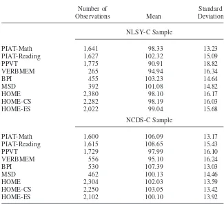
Table 1 presents summary statistics for the distribution of assessment scores in the two datasets. In the NLSY-C, some of the assessments were given to a wider age
420 The Journal of Human Resources
Table 1
Descriptive Statistics on Scores on Child Assessments, NLSY-C and NCDS-C, Normed to U.S. Population
Number of Standard
Observations Mean Deviation
NLSY-C Sample
PIAT-Math 1,641 98.33 13.23
PIAT-Reading 1,627 102.32 15.09
PPVT 1,775 90.91 18.82
VERBMEM 265 94.94 16.34
BPI 455 103.23 14.64
MSD 392 101.08 14.82
HOME 2,380 98.10 16.17
HOME-CS 2,282 98.19 16.03
HOME-ES 2,022 99.04 15.68
NCDS-C Sample
PIAT-Math 1,600 106.09 13.17
PIAT-Reading 1,615 108.65 15.43
PPVT 1,729 97.99 16.10
VERBMEM 556 95.10 16.24
BPI 530 107.39 13.03
MSD 462 100.13 14.46
HOME 2,304 102.03 13.59
HOME-CS 2,250 103.05 13.42
HOME-ES 2,102 100.10 13.92
Note: Based on those observations with a valid HOME score. For both countries, the scores were normed against external nationally representative samples of U.S. children, in which scores were standardized to have a mean of 100 and a standard deviation of 15. The exception to this is the HOME scores. Because there is no appropriate external sample available for HOME scores, in the NLSY-C they are standardized, by age, to have a mean of 100 and a standard deviation of 15 for each given year and in the NCDS-C scores are then normed with respect to the NLSY-C scores.
range than in the NCDS-C. To maintain comparability and avoid implicitly selecting samples that differ in terms of the age of mother—a variable that is likely to be endogenous with respect to child development outcomes—we restrict our samples to the intersection of the age ranges for each assessment: Those who are five years and older for the PIATs, four years and older for PPVT, four years old until the age of seven for verbal memory and BPI, and birth to four years for MSD. The varia-tion in age range for these tests also implies that cauvaria-tion is warranted in any cross-assessment comparisons.
surveys, known as the HOME score, which is designed to evaluate the quantity and quality of resources available for the child at home; this variable will play a key role in the multivariate analysis that follows. The HOME score, which comes from a series of questions asked of the child’s mother and interviewer observations about the child’s home, can be broken into two subscales. The first gauges the level of cognitive stimulation in the child’s home [HOME-CS] and the second measures the degree of emotional support there [HOME-ES]. While the surveys do not directly measure the purchase of goods and services that may aid in the child’s development, the relationship between income and the HOME scores can help assess the degree to which additional financial resources enable an improvement in a child’s home environment, either through direct spending or, indirectly, by alleviating the emo-tional strains of economic hardship. Spending on the child that occurs outside the home—for example, to improve the quality of education or child care—is, however, less likely to be captured by HOME measures. In contrast to the child assessments, an appropriate external sample for norming the HOME scores is not available, so the NLSY-C transforms each year’s raw HOME scores by age to have a mean of 100 and a standard deviation of 15. We have employed the parameters used in the transformation of the NLSY-C raw scores to standardize the raw scores in the NCDS-C with respect to the distribution in the NLSY-C.
The mean cognitive assessment scores shown in Table 1 for the NCDS-C are higher than those for the NLSY-C, though barely so for verbal memory, consistent with the patterns described by Michael (1999). Keeping in mind that a lower BPI is preferable to a higher one, the U.S. scores are superior to the British ones for the two noncognitive scales, though as with the cognitive assessments, the differences are small and never statistically significant. For the HOME scores, the averages for the British sample are slightly higher than those for the U.S. sample.
422 The Journal of Human Resources
For permanent income, after converting 1981 income into 1991 pounds using the retail prices index, we average over the two years, provided incomes are available for both. The average dollar/pound exchange rate prevailing in 1991 is then used to convert both measures of income into 1991 dollars.
In the NLSY-C, information is reported on income on a range of sources over the entire past calendar year. Included as income is money received from food stamps, an in-kind benefit, which has no British equivalent.4No other kind benefits are
in-cluded for either country, as either an absence of essential data or thorny valuation problems makes it precarious to impute to individual families values for housing subsidies or publicly provided health insurance. The family income variable consists of the income of the respondent and her spouse or partner; that is, income from other adults in the household is excluded for greater comparability with the measure available in the NCDS-C. As in most datasets for the United States, the total fam-ily income variable that results from summing income from these sources is pre-tax but post-transfer. As income after taxes and transfers is a better measure of the re-sources in a family’s control and more comparable to the income measures in the NCDS-C, we impute tax liability using information from the March Current Popula-tion Survey (CPS) and net taxes out.5After converting 1981 income to a 1991 basis
using the CPI-U, after-tax income for the two years, if both are available, is then averaged to form a measure of permanent income.6For both countries, to avoid any
undue influence of outliers, any annual income variables exceeding $100,000 were top-coded at $100,001, and the few cases where negative income was reported were ‘‘bottom-coded’’ at zero.
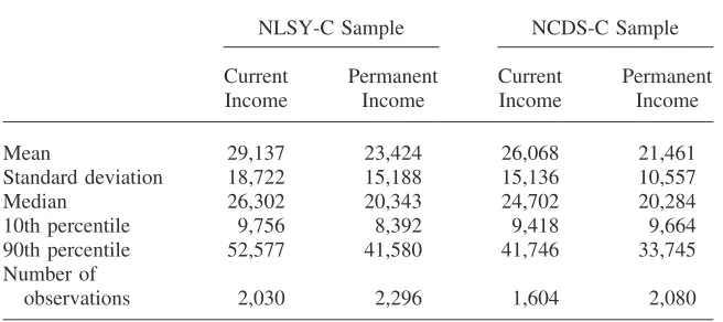
Table 2 presents descriptive statistics on the distribution of income from the two samples. For both income measures, the mean and median levels are somewhat higher in the U.S. sample than in the British sample, with the gap in means being somewhat greater than that for the medians. Consistent with other rankings of coun-try by inequality (for example, Gottschalk and Smeeding 1997), there is also greater dispersion of income in the NLSY-C than in the NCDS-C, as measured by the ratio of the 90th to the 50th percentile or the 50th percentile to the 10th percentile. Overall, though, these differences are small, and, with respect to the distribution of income, the two samples show a high degree of similarity.
4. Though attempts are sometimes made to impute a market value to food stamps, analysts often consider them to be close enough to cash to be counted as such (Moffitt 2000).
5. The March CPS contains respondent-generated information on pre-tax, post-transfer income and impu-tations for liabilities for federal, state and social security taxes that are generated by the U.S. Census Bureau’s tax model. We first use the CPS data to estimate a regression model where the tax liabilities of a tax unit are a function of variables describing income and family structure. The coefficients thereby generated are then combined with characteristics taken from the NLSY-C to predict the tax bill of each family. This procedure is done separately for 1981 and 1991.
Table 2
Descriptive Statistics on Income Measures, NLSY-C and NCDS-C
NLSY-C Sample NCDS-C Sample
Current Permanent Current Permanent
Income Income Income Income
Mean 29,137 23,424 26,068 21,461
Standard deviation 18,722 15,188 15,136 10,557
Median 26,302 20,343 24,702 20,284
10th percentile 9,756 8,392 9,418 9,664
90th percentile 52,577 41,580 41,746 33,745
Number of
observations 2,030 2,296 1,604 2,080
Notes: Income is reported in 1991 dollars and only for those observations with a valid HOME score. Each permanent income measure is calculated by averaging income over the years 1981 and 1991 for which it is available.
IV. Empirical Specifications
Our main goal is to identify for both countries the effect of exogenous changes in income on measures of child development. One approach would be to estimate a structural model where the household maximizes utility over consumption, leisure, and the achievement of its children, and has a production function that trans-lates inputs of time and other resources into achievement levels. Estimation of such a model would require making strong assumptions, especially in light of the fact that the datasets used contain almost no information on family expenditures for such categories as books or health care, or on how time outside of work is spent (Blau 1999).
424 The Journal of Human Resources
in the same way across the two datasets, but data restrictions make some differences necessary. To account for the greater ethnic and racial diversity in the NLSY-C than in the NCDS-C, additional controls for race and ethnicity are included in the set of ‘‘core’’ regressors for the NLSY-C.7
Mother’s scores on standardized tests also are included in some specifications in an attempt to control for ability. Although it is desirable to include such measures to avoid attributing to income the impact of the mother’s abilities that affect earnings power as well as child development, the test scores may capture both innate ability, and endogenous decisions by the mother regarding her own human capital invest-ment. In the NLSY, the scores used in the regressions are from four of the sections of the Armed Services Vocational Aptitude Battery (ASVAB): arithmetic reason-ing, word knowledge, paragraph comprehension, and numerical operations.8In the
NCDS, the aptitude measures used are reading and math scores from a standardized test taken in school at age 16.
The following linear specification is used:
(1) Aij⫽Xjβi⫹Ijαi⫹εij
where Aij is the jth child’s score on theith child assessment,Xis a vector of re-gressors,Iis the measure of income,εis the disturbance term, andαandβare the parameters of the models. The models are estimated by ordinary least squares (OLS). Results from three specifications are reported. In the first,Xconsists of no variables. In the second,Xis made up of the core regressors. In the third specification,Xis composed of the core regressors and the mother’s test scores. In each case, the stan-dard errors have been corrected for the fact that a mother often has more than one child represented in the samples.
While we are careful about the variables we include in the specifications, it is difficult to go further in addressing econometric problems arising from the endogene-ity of income because of limitations inherent in the NCDS-C. When analyzing the NLSY-C, Blau (1999) is able to use the presence in the data of children who are assessed more than once, of siblings, and of first cousins to estimate fixed-effect models. These models will generate consistent estimates, assuming that any unob-servables that are correlated with income and have an impact on child outcomes are fixed within the relevant group of observations—the individual over different time periods, siblings, or cousins—and can therefore be differenced out. In the NCDS-C, it is not possible to estimate such models; though it is often the case that more than one child in the family has been assessed, the tests were taken at the same time, implying no within-family variation in income. Thus, while we will not present re-sults from any techniques other than OLS, it is worth remembering that findings from the United States suggest that OLS overstates the impact of income on child development.
In addition, measurement error may impact the estimated income effects. Current income is likely to mismeasure the true level of family resources because of the variation in earnings over the life cycle and misreporting by respondents. While a
7. Definitions of all regressors can be found in an appendix that is available upon request.
multiple-year average of income should be measured with less error than a single year of income, some degree of measurement error will persist.9Moreover, because
the parameters of the distribution of misreporting and the mobility of income over the lifecycle are likely to differ across the two countries, the extent to which the attenuation bias diminishes when one moves from the current to the permanent in-come measure will vary across the datasets, making direct comparisons of the U.S. and British results somewhat tenuous.
V. Results
In this section, we first present results from our basic specifications. We then explore whether there is evidence of nonlinearities in the relationship be-tween income and the assessments. Finally, we turn to a preliminary examination of differences between the two nations regarding the routes by which family income affects child outcomes.
A. Main Results
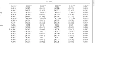
Table 3 presents OLS results for both income measures from the three specifications of Equation 1. As the table reports the results of 72 different regressions, a few words of orientation may be helpful. Columns 1 through 3 report the estimated effects for current income and Columns 4 through 6 report their counterparts for permanent income. The estimates from the NLSY-C are reported in the top half of the tables and those using the NCDS-C are provided in the bottom half. In the regression analy-sis, the normed scores for each country are divided by the standard deviation of the external U.S. population (15). Because the units of income are 10,000’s of 1991 U.S. dollars, the coefficients measure the change in assessment score (in standard deviations in a representative U.S. population) with respect to a $10,000 change in current or permanent income. As mentioned, lower scores are preferable to higher ones for BPI, while the opposite is true for the other five assessments. The relation-ship between the motor and social development assessment and family income may be limited by ‘‘ceiling effects’’ as scores on this assessment frequently top out for the older children (Baker et al. 2001).
We can obtain a first look at how the effects of income on child development in Great Britain match up to those in the United States by comparing the coefficients in the top and bottom halves of Column 1, which summarize the results of specifica-tions where current income is the only explanatory variable. In the NCDS-C, the results for the four cognitive tests are quite similar: All coefficients are significant at the 1 percent level and are in the narrow range of 10.0 percent (verbal memory) of a standard deviation to 14.0 percent (PPVT). The results for the cognitive assess-ments in the United States are broadly similar, with the exception of the fact that there is no evidence of financial resources making a difference with respect to scores on the verbal memory assessment. For the remaining three cognitive assessments,
426
The
Journal
of
Human
Resources
Table 3
OLS Regression Coefficients on Current and Permanent Income, NLSY-C and NCDS
Current Income Permanent Income
Income Core⫹ Income Core⫹
Specification Only Core Test Scores Only Core Test Scores
Assessment NLSY-C
PIAT-Math 0.146** 0.090** 0.058** 0.178** 0.104** 0.067**
(n⫽1,423) (0.016) (0.015) (0.015) (0.021) (0.019) (0.018)
[0.082] [0.167] [0.203] [0.080] [0.162] [0.202]
PIAT-Reading 0.149** 0.096** 0.054** 0.179** 0.104** 0.055*
(n⫽1,410) (0.020) (0.019) (0.018) (0.029) (0.026) (0.024)
[0.067] [0.137] [0.199] [0.063] [0.131] [0.197]
PPVT 0.230** 0.123** 0.075** 0.272** 0.132** 0.074*
(n⫽1,546) (0.025)o (0.023) (0.021) (0.033) (0.029) (0.027)
[0.101] [0.262] [0.322] [0.094] [0.255] [0.319]
Verbal memory 0.026 0.052 0.012 0.039 0.059 0.024
(n⫽245) (0.039) (0.049) (0.049) (0.053) (0.065) (0.066)
[⫺0.002] [0.046] [0.046] [⫺0.001] [0.045] [0.047]
BPI ⫺0.085** ⫺0.088** ⫺0.077** ⫺0.096** ⫺0.098** ⫺0.084*
(n⫽417) (0.025) (0.027) (0.028) (0.031) (0.034) (0.035)
[0.027] [0.049] [0.057] [0.024] [0.043] [0.053]
MSD 0.028 0.017 0.017 0.030 0.006 0.007
(n⫽395) (0.022) (0.026) (0.027) (0.027) (0.030) (0.030)
Aughinbaugh
and
Gittleman
427
PIAT-Math 0.114** 0.091** 0.060** 0.193** 0.165** 0.117**
(n⫽1,169) (0.021) (0.021) (0.020) (0.028) (0.028) (0.027)
[0.030] [0.086] [0.161] [0.044] [0.098] [0.168]
PIAT- Reading 0.118** 0.101** 0.065** 0.200** 0.181** 0.122**
(n⫽1,187) (0.023) (0.023) (0.021) (0.031) (0.031) (0.029)
[0.026] [0.074] [0.157] [0.037] [0.085] [0.162]
PPVT 0.140** 0.122** 0.082** 0.226** 0.201** 0.139**
(n⫽1,265) (0.026)° (0.026) (0.023) (0.036) (0.036) (0.034)
[0.032] [0.083] [0.160] [0.044] [0.092] [0.164]
Verbal memory 0.100** 0.088* 0.054 0.142** 0.131* 0.078
(n⫽408) (0.030) (0.032) (0.032) (0.043) (0.044) (0.042)
[0.016] [0.071] [0.100] [0.018] [0.074] [0.101]
BPI ⫺0.068* ⫺0.067 ⫺0.065 ⫺0.068 ⫺0.059 ⫺0.048
(n⫽383) (0.032) (0.034) (0.035) (0.042) (0.042) (0.043)
[0.010] [⫺0.015] [⫺0.009] [0.005] [⫺0.021] [⫺0.016]
MSD 0.038 0.042 0.054 0.039 0.050 0.060
(n⫽346) (0.029) (0.031) (0.032) (0.032) (0.040) (0.041)
[0.002] [0.083] [0.094] [0.000] [0.081] [0.091]
Notes: Standard errors in parentheses. Adjusted R2in square brackets. Coefficients measure the effect on the assessment score (in standard deviations) of a change in
428 The Journal of Human Resources
the magnitudes of the (significant) coefficients are somewhat higher in the United States than Great Britain (14.6 percent to 23.0 percent).
Little difference between the two countries is evident in the results for the non-cognitive tests. Higher income levels are associated with some reduction in be-havioral problems but do not appear to have any impact on motor and social development.
If one ignores the possibility of measurement error, the results in Column 1 are likely to provide an upper bound on the impact ofcurrentincome, as no account is taken of observable or unobservable factors that are correlated with both income and the child development outcomes. The largest impact of a change in $10,000— which is about one-half of a standard deviation of current income in the U.S. sample, and about two-thirds of one in the British sample—is below one-quarter of a standard deviation, and most of the measured impacts are substantially smaller than that.
Further perspective on the size of the elasticity of assessment scores with respect to income can be provided by putting these numbers into a policy context.10 For
instance, a $10,000 increase in income is much larger than the largest transfer pro-vided by the Earned Income Tax Credit (EITC), let alone any increase in EITC generosity that is likely to be contemplated in the coming years. In 2000, a low-income family with two children could have received as much as $3,888 from the EITC program, provided earnings fell below $12,700. Given that this EITC maxi-mum is worth $3,075 in 1991 dollars, the largest coefficient in Column 1 for the United States, that for PPVT, implies that EITC receipt would increase test scores by about 7 percent of a standard deviation (0.230*$3,075/$10,000). Under the as-sumption that the standardized test scores have a normal distribution, this impact implies that the test score of a child starting at the median would rise above an additional 2.8 percent of the population, or that a child at the first quartile would move to roughly the 27th percentile.
In-work benefits in the United Kingdom are more generous, but, given the smaller estimated coefficients, imply effects that are not much larger. A family with two children could have received up to £8,139 from the Working Families Tax Credit (WFTC) in 2000, though this amount overstates the net gain to the family from WFTC as the credit counts as income when computing entitlement for housing and other benefits (Blundell and Hoynes 2001). Using an exchange rate of £1⫽$1.50 and deflating implies a credit of $6,437 in 1991 dollars. Here the PPVT coefficient (0.140) suggests that those children originally scoring at the median will rise above an additional 3.6 percent of the population, while those at the 25th percentile will move to nearly the 28th percentile.
Although caution is warranted in comparing the magnitudes of the income effects across countries, given the unavoidable discrepancies in the income concepts and the likelihood that any bias from income measurement error differs across the two surveys, we have calculated whether the estimated income effects are significantly different, and have marked these cases on Table 3 using the symbol ‘‘°’’. For the first column of results, PPVT is the only case where such a difference is statistically
significant at the 5 percent level and, it is, in fact, the only such instance for all the cross-country comparisons in the entire paper.
When the family background variables that make up the core set of regressors are added to the specification (Column 2), the results change little qualitatively, but there is almost always a reduction in the magnitude of the measured impact, particu-larly for the effects of income on cognitive assessment scores in the United States. As a result, the gap between the two countries’ coefficients are narrower than for the first specification, though it is now the case that the effects in Great Britain are slightly larger.
As the core regressors do not include a control for ability, the estimates from Specification 2 probably continue to overstate the impact of current income. At this stage, we add test scores to the specification, acknowledging that these scores may be a product not only of innate ability and family background, but also to some extent the result of endogenous decisions made by the mother with respect to her human capital investment. The addition of this set of variables further reduces the estimates of the current income effect by roughly an additional 30-40 percent across the variouscognitivetest scores in both datasets, owing to a high correlation between income and the mother’s scholastic ability. All income effects estimated based on this third specification are quite small, the largest being 8.2 percent of a standard deviation.
When permanent income is used as a measure of resources, there is very little qualitative change in the results. For both countries, the results continue to point to a positive relationship between income and all cognitive assessments except for verbal memory, although greater financial resources continue to be associated with higher scores on the verbal memory assessment in Great Britain. There is, however, a no-ticeable cross-national difference with respect to the magnitudes of the changes in coefficients in regressions for the cognitive assessments. For example, comparing the first specifications across the income measures (Columns 1 and 4), the effect of permanent income on PIAT-Math, PIAT-Reading and PPVT scores in Great Britain is about 60–70 percent higher than that for current income, while for the United States the corresponding increases are 18–22 percent. In fact, with this relatively small amount of change between the two income concepts, after adding controls for the core regressors and test scores, it is hard to distinguish the permanent income results in the United States from the corresponding current income results. That is less the case in Great Britain, where the current income effects ranged from 5.4 percent to 8.2 percent of a standard deviation on the cognitive assessments, while the permanent income impacts now run from 7.8 percent to 13.9 percent.
430 The Journal of Human Resources
fluctuations, movements into and out of the labor force, and changes in household composition.11
Leaving aside the question of cross-country differences, the main message of the results in Table 3 is that there is little evidence to support the hypothesis that assess-ment scores respond strongly to income changes. Our own examination (not pre-sented) and that of Blau (1999) shows that this picture does not change much for the United States if additional years of data are used to calculate permanent income. A couple of calculations may serve to put the magnitudes further into context. First, in the specifications with core controls and mother’s test scores, the largest increase associated with a $10,000 increase in income (0.139 standard deviations) can be translated into a movement beyond 5.5 percent of the population if starting from the median, 4.6 percent from the first quartile, and 2.7 percent from the first decile.
Second, in the NCDS-C sample, the factor with the largest impacts on test scores is the occupational class of the child’s maternal grandfather. Specifications where the only regressors are dummy variables representing this occupation imply an in-crease in score ranging from 27 percent to 101 percent of a standard deviation when one shifts from the lowest-ranked occupation (on the basis of the corresponding score) to the highest one, and a gain that is 52 percent of a standard deviation or greater for five out of six scores. In contrast, the comparable Specification 1 results show that the largest impact of a $10,000 increase in our measures of a family’s financial resources is 14 percent of a standard deviation for current income and 23 percent for permanent income.
In the NLSY-C, grandfather’s occupation also appears to have stronger effects than does income. A shift from the lowest occupational class to the highest is associ-ated with an increase in test scores of 14 percent to 73 percent of a standard deviation, and a gain of at least 39 percent of a standard deviation for five of the six scores. For five of the six outcomes, the gain from grandfather’s occupation is about twice that for an additional $10,000 in current income or permanent income.12
B. Nonlinearities in Income Effects
The possibility that the effect of income on child development may diminish as income rises is an issue that has been prominent in the literature (Duncan and Brooks-Gunn 1997; Mayer 1997; Blau 1999). If such nonlinearities exist, then they would likely serve to raise the average effect of income somewhat more in the United States than in Great Britain, as the former has a greater proportion of children living in low-income households.
11. The patterns describing income effects and cross-country differences are, however, robust to the factors we could examine by restricting the samples to those: 1) with income data available for both 1981 and 1991; 2) whose marital status is the same in 1981 and 1991; and 3) whose educational qualifications do not change from 1981 to 1991.
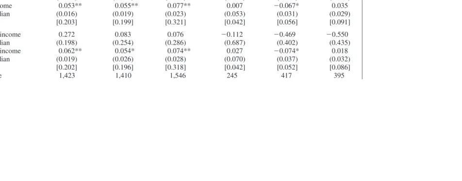
Table 4 presents OLS results for spline regressions based on Specification 3, esti-mated to examine the presence of nonlinearities in the impact of income. One-half of median family income, a cutoff that has been used as a poverty line in international comparisons (Smeeding, O’Higgins, and Rainwater 1990), serves as the ‘‘knot’’ in these piecewise-linear regressions. In the NLSY-C data, 20 percent and 18 percent of the sample has income below half the median measured using current and permanent income, respectively. Because of a lower degree of income inequality, smaller por-tions of the NCDS-C sample, 12 percent for current income and 10 percent for per-manent, fall below one-half of the median.
The spline results provide little evidence of diminishing marginal returns of in-come for child development. For the current inin-come results, it is more common for the coefficient for income for those in poverty to be of the ‘‘wrong’’ sign in the NCDS-C sample—that is, implying that additional resources worsen child develop-ment outcomes—than it is for this coefficient to be larger in size that its counterpart for those above one-half the median, as would be consistent with the presence of nonlinearities in the relationship between income and child development. In the NLSY-C, though the effect of current income for those in poverty is, in most cases, larger than the effect of income for those above one-half the median, the difference in the estimated income effects is statistically different only for motor and social development, where the effect of income is much smaller, and even negative for those with income below one-half the median.
For the permanent income regressions, the magnitudes are consistent with the diminishing returns story for the four cognitive assessments using the NCDS-C and for three of the four cognitive assessments and BPI using the NLSY-C, but the differ-ences in the impact of income above and below the knot is never statistically signifi-cant in these cases. As already indicated, moreover, despite the presence of some variance in the patterns across countries, it is never the case that the cross-national differences in coefficient magnitudes are statistically significant.
432
The
Journal
of
Human
Resources
Table 4
Spline Regression Coefficients on Current and Permanent Income, NLSY-C and NCDS, Knot at 0.5 * Median
PIAT- PIAT- Verbal
Assessment Math Reading PPVT Memory BPI MSD
Specification NLSY-C
Current income 0.167 0.051 0.027 0.103 ⫺0.300 0.426
⬍.5*median (0.115) (0.144) (0.166) (0.384) (0.287) (0.235)
Current income 0.053** 0.055** 0.077** 0.007 ⫺0.067* 0.035
ⱖ.5*median (0.016) (0.019) (0.023) (0.053) (0.031) (0.029)
[0.203] [0.199] [0.321] [0.042] [0.056] [0.091]
Permanent income 0.272 0.083 0.076 ⫺0.112 ⫺0.469 ⫺0.550
⬍.5∗median (0.198) (0.254) (0.286) (0.687) (0.402) (0.435)
Permanent income 0.062** 0.054* 0.074** 0.027 ⫺0.074* 0.018
ⱖ.5∗median (0.019) (0.026) (0.028) (0.070) (0.037) (0.032)
[0.202] [0.196] [0.318] [0.042] [0.052] [0.086]
Aughinbaugh
and
Gittleman
433
Current income ⫺0.016 ⫺0.112 0.138 ⫺0.361 ⫺0.064 ⫺0.220
⬍.5∗median (0.159) (0.168) (0.174) (0.215) (0.248) (0.264)
Current income 0.066** 0.077** 0.079** 0.082* ⫺0.065 0.070*
ⱖ.5∗median (0.022) (0.023) (0.025) (0.038) (0.039) (0.036)
[0.160] [0.157] [0.159] [0.103] [⫺0.012] [0.094]
Permanent income 0.290 0.102 0.576 0.117 0.213 ⫺0.502
⬍.5∗median (0.256) (0.275) (0.371) (0.416) (0.426) (0.439)
Permanent income 0.110** 0.123** 0.121** 0.077 ⫺0.058 0.082
ⱖ.5∗median (0.030) (0.031) (0.036) (0.045) (0.047) (0.045)
[0.167] [0.161] [0.165] [0.098] [⫺0.018] [0.092]
Sample size 1,169 1,187 1,265 408 383 346
Notes: Standard errors in parentheses. Adjusted R2in square brackets. Coefficients measure change in score (in standard deviations) with respect to a change in income
434 The Journal of Human Resources
C. Does Income Affect Child Development Differently Across the Two Countries?
Up until this point, most of the evidence points to a strong resemblance between the two countries in the relationship between income on child development. We are also interested in assessing whether the countries are similar with respect to the pathways through which income influences childhood development. While a detailed examination of this question is beyond the scope of this paper and is, in any case, constrained by a lack of data on the extent to which parents devote money and time to their children, we will address two issues with regard to the character of the income–child development link.
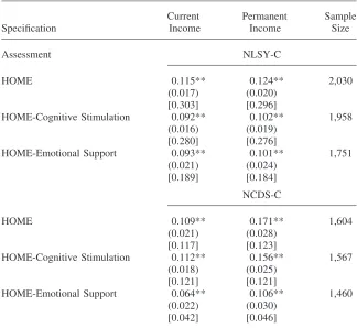
First, the child development literature has recently sought to distinguish between routes by which the income of a family may influence its children’s development (Guo and Harris 2000; Yeung, Linver, and Brooks-Gunn 2001). A perspective re-ferred to as the ‘‘human capital’’ or ‘‘financial resources’’ model emphasizes that money can be invested in the development of the child, whether it be used to improve the physical environment for learning, to ensure the child remains in good health, or to purchase goods and services that will aid in cognitive stimulation. An alternative perspective emphasizes the emotional impact that economic hardship has on parent-child interactions, for example, through heightened levels of stress or a greater likeli-hood of parental depression. As noted above, both datasets contain a measure of the quantity and quality of resources in the child’s home (HOME), which can be divided into subscales for cognitive stimulation CS) and emotional support (HOME-ES). As HOME-CS includes information about the quality of the physical environ-ment and measures the presence of educational materials such as books, trips to museums, and time spent teaching the child her letters or numbers, a positive rela-tionship between HOME-CS and the assessment scores would be consistent with resources, in and of themselves, being important. An analogous relationship between HOME-ES and performance on the assessments would underscore the significance of a family’s psychological well-being and interactions with the child.
Clearly, financial resources may influence child development via routes that do not pass through the home. For example, higher income may enable access to better quality schooling or child care. In addition, there may be other investments in chil-dren that occur inside the home, but are not captured in HOME and its subscales. In the absence of complete measures, one can infer that additional investments are occurring, if income continues to have a significant relationship to the assessments, after controlling for the home environment.
Table 5
OLS Regression Coefficients of Home Scores on Income, NLSY-C and NCDS
Current Permanent Sample
Specification Income Income Size
Assessment NLSY-C
HOME 0.115** 0.124** 2,030
(0.017) (0.020)
[0.303] [0.296]
HOME-Cognitive Stimulation 0.092** 0.102** 1,958
(0.016) (0.019)
[0.280] [0.276]
HOME-Emotional Support 0.093** 0.101** 1,751
(0.021) (0.024)
[0.189] [0.184]
NCDS-C
HOME 0.109** 0.171** 1,604
(0.021) (0.028)
[0.117] [0.123]
HOME-Cognitive Stimulation 0.112** 0.156** 1,567
(0.018) (0.025)
[0.121] [0.121]
HOME-Emotional Support 0.064** 0.106** 1,460
(0.022) (0.030)
[0.042] [0.046]
Notes: Standard errors in parentheses. Adjusted R2in square brackets. Coefficients measure the effect on
HOME score (in standard deviations) of a change in income of $10,000 1991 dollars. Each regression includes the core regressors and test scores. Inclusion in ‘‘permanent’’ sample requires presence in ‘‘cur-rent’’ one. * indicates the coefficient is significant at the 5 percent level, ** at the 1 percent level.
436
The
Journal
of
Human
Resources
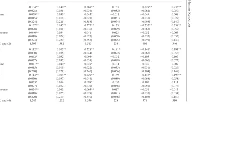
Table 6
OLS Regression Coefficients from HOME Specifications
PIAT- PIAT- Verbal
Math Reading PPVT Memory BPI MSD
A. NLSY-C
(1) HOME 0.134** 0.140** 0.269** 0.133 ⫺0.229** 0.235** (0.028) (0.031) (0.036) (0.082) (0.062) (0.059) Current income 0.039** 0.036* 0.043* ⫺0.011 ⫺0.049 0.008
(0.015) (0.018) (0.021) (0.051) (0.031) (0.027) [0.224] [0.221] [0.353] [0.074] [0.093] [0.140] (2) HOME 0.137** 0.145** 0.275** 0.123 ⫺0.235** 0.238**
(0.028) (0.031) (0.036) (0.079) (0.061) (0.059) Permanent income 0.046** 0.034 0.041 0.023 ⫺0.052 ⫺0.003
(0.018) (0.024) (0.027) (0.068) (0.037) (0.032) [0.223] [0.220] [0.352] [0.075] [0.091] [0.140] Sample size (1) and (2) 1,395 1,382 1,513 238 401 346
(3) HOME-CS 0.112** 0.102** 0.228** 0.181* ⫺0.141* 0.191** (0.030) (0.036) (0.044) (0.092) (0.068) (0.058) HOME-ES 0.062* 0.052 0.098* ⫺0.032 ⫺0.105 0.107
(0.027) (0.033) (0.039) (0.088) (0.060) (0.073) Current income 0.041** 0.040* 0.049* ⫺0.014 ⫺0.040 0.007
(0.015) (0.019) (0.022) (0.053) (0.031) (0.029) [0.220] [0.221] [0.340] [0.066] [0.104] [0.149] (4) HOME-CS 0.113** 0.104** 0.229** 0.169 ⫺0.143* 0.193**
(0.030) (0.037) (0.044) (0.089) (0.068) (0.058) HOME-ES 0.063* 0.054 0.099* ⫺0.033 ⫺0.105 0.111
(0.027) (0.032) (0.039) (0.088) (0.059) (0.073) Permanent income 0.054** 0.043 0.063** 0.017 ⫺0.051 ⫺0.013
Aughinbaugh
and
Gittleman
437
(1) HOME 0.139** 0.169** 0.228** 0.133 ⫺0.192** 0.161** (0.032) (0.035) (0.037) (0.072) (0.060) (0.059) Current income 0.043** 0.050* 0.054* 0.054 ⫺0.055 0.039
(0.021) (0.020) (0.022) (0.033) (0.036) (0.034) [0.177] [0.188] [0.202] [0.132] [0.005] [0.096] (2) HOME 0.131** 0.163** 0.223** 0.135 ⫺0.201** 0.163**
(0.032) (0.035) (0.037) (0.072) (0.060) (0.059) Permanent income 0.090** 0.092** 0.093* 0.072 ⫺0.031 0.036
(0.028) (0.028) (0.033) (0.044) (0.044) (0.042) [0.181] [0.190] [0.204] [0.132] [⫺0.002] [0.093] Sample size (1) and (2) 1,119 1,135 1,206 380 361 319
(3) HOME-CS 0.093* 0.161** 0.197** 0.121 ⫺0.180** 0.126* (0.039) (0.041) (0.044) (0.075) (0.068) (0.063) HOME-ES 0.091** 0.054 0.094* 0.071 ⫺0.095 0.064
(0.032) (0.038) (0.037) (0.067) (0.051) (0.066) Current income 0.040 0.044* 0.045 0.048 ⫺0.048 0.057
(0.023) (0.022) (0.023) (0.033) (0.035) (0.039) [0.174] [0.187] [0.197] [0.128] [0.017] [0.089] (4) HOME-CS 0.089* 0.157** 0.194** 0.123 ⫺0.185** 0.133* (0.039) (0.041) (0.044) (0.074) (0.068) (0.063) HOME-ES 0.087** 0.051 0.091* 0.070 ⫺0.099 0.065
(0.032) (0.038) (0.037) (0.067) (0.051) (0.066) Permanent income 0.086** 0.085** 0.087* 0.075 ⫺0.032 0.038
(0.029) (0.030) (0.036) (0.045) (0.043) (0.049) [0.179] [0.190] [0.200] [0.129] [0.013] [0.083] Sample size (3) and (4) 1,024 1,039 1,111 368 351 269
Notes: Standard errors in parentheses. Adjusted R2in square brackets. Coefficients measure the effect on the assessment score (in standard deviations) of a one standard
438 The Journal of Human Resources
no case are the cross-country differences in impacts statistically significant, some-thing that is true for all the coefficients contained in Table 6.
Of more interest perhaps are estimates of the relative importance of cognitive stimulation and emotional support. In both surveys, the impact of an increase in HOME-CS exceeds that of HOME-ES. HOME-CS raises the outcomes by between 10 percent and 23 percent in the NLSY-C and is significant for all outcomes except verbal memory, while HOME-ES is significant only for PIAT-Math and PPVT. In the NCDS-C, the effects of HOME-CS range from 9 percent to 20 percent, and again this variable is not consistently significant for verbal memory. HOME-ES is consistently significant for the same assessments as for the NLSY-C.
Our finding that the cognitive environment tends to be more important than the emotional one in child development is broadly consistent with the results of Yeung, Linver, and Brooks-Gunn (2001) and Guo and Harris (2000). Finally, it is clear from Table 6 that, even after taking account of the HOME scores, income still plays a role, albeit a reduced one, in improving the scores on the assessments, particularly the PIAT-Math, PIAT-Reading and PPVT. This finding provides support for the notion that there are other routes not captured by the HOME measures by which higher income benefits children.
VI. Conclusions
Recent research that has paid careful attention to the difficult econo-metric issues present when investigating the question of whether money impacts child development has come to the conclusion that, in the United States, money matters, but to a small extent. In this paper, we have examined the relationship be-tween income and child development using U.S. and British data, and found that the recent findings for the United States carry over to Great Britain. For both nations, income does tend to improve cognitive test scores, but the magnitude of the impact is small. For noncognitive outcomes, the results are also similar for both countries. Higher levels of income are associated with a reduction in child behavior problems, but seem to have little impact on motor and social development. The countries also exhibit a strong resemblance in our cursory examination of the pathways by which money affects child development, with cognitive stimulation tending to be of greater importance than emotional support, and income continuing to show some effect, mainly on the cognitive assessments, after including controls for the home environ-ment.
social welfare policies than either of these two nations, does money matter more? On the other, are the effects of family income negligible in countries such as those in Scandinavia where the public sector is more active? Relatedly, in countries where public preschool care is widely available and educational quality varies less by in-come level, is it the case that inin-come, to the extent that it matters, impacts child development to a greater extent through improvements in the home environment, and to a smaller extent through the quality of education or child care outside the home?
References
Adema, Willem, Marcel Einerhand, Bengt Eklind, Jorgen Lotz, and Mark Pearson. 1996. ‘‘Net Public Social Expenditure.’’ Labour Market and Social Policy Occasional Papers No. 19. Paris: OECD.
Baker, Paula C., Canada K. Keck, Frank L. Mott, and Stephan V. Quinlan. 2001.NLSY
Child and Young Adult Handbook. Center for Human Resource Research, Ohio State University.
Bardasi, Elena, Stephen P. Jenkins, and John A. Rigg. 1999. ‘‘Documentation for Derived Current and Annual Net Household Income Variables, BHPS waves 1–7.’’ Essex: Uni-versity of Essex. Mimeo.
Blau, David M. 1999. ‘‘The Effect of Income on Child Development.’’Review of
Econom-ics and StatistEconom-ics81(2):261–76.
Blundell, Richard, and Hilary Hoynes. 2001. ‘‘Has ‘In-Work’ Benefit Reform Helped the Labour Market?’’ NBER Working Paper No. 8546.
Bo¨heim, Rene´, and Stephen P. Jenkins, 2000. ‘‘Do Current Income and Annual Income Measures Provide Different Pictures of Britain’s Income Distribution?’’ Essex: Univer-sity of Essex. Mimeo.
Brewer, Mike. 2000. ‘‘Comparing In-Work Benefits and Financial Work Incentives for Low-Income Families in the US and the UK.’’ Working Paper 00/16, The Institute for Fiscal Studies.
Currie, Janet. 2000. ‘‘Early Childhood Intervention Programs: What Do We Know?’’ Los Angeles: UCLA. Mimeo.
———. 1998. ‘‘The Effect of Welfare on Child Outcomes.’’ InWelfare, the Family and
Reproductive Behavior: Research Perspectives, ed. Moffitt, Robert A., 177–204. Wash-ington, D.C.: National Academy Press.
Currie, Janet, and Duncan Thomas. 1999. ‘‘Early Test Scores, Socioeconomic Status, and Future Outcomes.’’ NBER Working Paper No. 6943.
Duncan, Greg J., and Jeanne Brooks-Gunn, eds. 1997.Consequences of Growing Up Poor.
New York: Russell Sage Foundation.
Gottschalk, Peter, and Timothy M. Smeeding. 1997. ‘‘Cross-National Comparisons of
Earn-ings and Income Inequality.’’Journal of Economic Literature35(2):633–87.
Guo, Guang, and Kathleen Mullan Harris. 2000. ‘‘The Mechanisms Mediating the Effects
of Poverty on Children’s Intellectual Development.’’Demography37(4):431–47.
Joshi, Heather, Elizabeth C. Cooksey, Richard D. Wiggins, Andrew McCulloch, Georgia Verropoulou, and Lynda Clarke. 1999. ‘‘Diverse Family Living Situations and Child De-velopment: A Multi-Level Analysis Comparing Longitudinal Evidence from Britain and
the United States.’’International Journal of Law, Policy, and the Family13(3):292–
314.
440 The Journal of Human Resources
Childhood Family Income on Completed Schooling.’’ Evanston: Northwestern Univer-sity. Mimeo.
Mayer, Susan 1997.What Money Can’t Buy: Family Income and Children’s Life Chances.
Cambridge: Harvard University Press.
Michael, Robert T. 1999. ‘‘Children’s Cognitive Skill Development in the U.S. and the U.K.’’ Chicago: University of Chicago. Mimeo.
Moffitt, Robert A. 2000. ‘‘Welfare Benefits and Female Headship in U.S. Time Series.’’ Baltimore: Johns Hopkins University. Mimeo.
Shea, John. 2000. ‘‘Does Parents’ Money Matter?’’Journal of Public Economics77(2):
155–84.
Smeeding, Timothy M., Michael O’Higgins, Lee Rainwater, eds. 1990.Poverty, Inequality
and Income Distribution in Comparative Perspective: The Luxembourg Income Study. Washington, D.C.: Urban Institute Press.