Calculus
Sixth Edition
Frank Ayres, Jr., PhD
Former Professor and Head of the Department of Mathematics
Dickinson College
Elliott Mendelson, PhD
Professor of Mathematics
Queens College
Schaum’s Outline Series
ELLIOTT MENDELSON, PhD, is professor of mathematics at Queens College. He is the author of Schaum’s Outline of Beginning Calculus.
Copyright © 2013 The McGraw-Hill Companies, Inc. All rights reserved. Except as permitted under the United States Copyright Act of 1976, no part of this publication may be reproduced or distributed in any form or by any means, or stored in a database or retrieval system, without the prior written permission of the publisher.
ISBN: 978-0-07-179554-8 MHID: 0-07-179554-5
The material in this eBook also appears in the print version of this title: ISBN: 978-0-07-179553-1, MHID: 0-07-179553-7.
All trademarks are trademarks of their respective owners. Rather than put a trademark symbol after every occurrence of a trademarked name, we use names in an editorial fashion only, and to the benefi t of the trademark owner, with no intention of infringement of the trademark. Where such designations appear in this book, they have been printed with initial caps.
McGraw-Hill eBooks are available at special quantity discounts to use as premiums and sales promotions, or for use in corporate training programs. To contact a representative please e-mail us at [email protected].
McGraw-Hill, the McGraw-Hill Publishing logo, Schaum’s, and related trade dress are trademarks or registered trademarks of The McGraw-Hill Companies and/or its affi liates in the United States and other countries and may not be used without written permission. All other trademarks are the property of their respective owners. The McGraw-Hill Companies is not associated with any product or vendor mentioned in this book.
TERMS OF USE
This is a copyrighted work and The McGraw-Hill Companies, Inc. (“McGraw-Hill”) and its licensors reserve all rights in and to the work. Use of this work is subject to these terms. Except as permitted under the Copyright Act of 1976 and the right to store and retrieve one copy of the work, you may not decompile, disassemble, reverse engineer, reproduce, modify, create derivative works based upon, transmit, distribute, disseminate, sell, publish or sublicense the work or any part of it without McGraw-Hill’s prior consent. You may use the work for your own noncommercial and personal use; any other use of the work is strictly prohibited. Your right to use the work may be terminated if you fail to comply with these terms.
Check out the full range of Schaum resources available from McGraw-Hill Education.
At
Schaums.com
, you’ll find videos for
all the most popular Schaum’s subjects
Watch and hear instructors explain
problems step by step
Learn valuable problem-solving
techniques
Find out how to tackle common
problem types
Get the benefits of a real
classroom experience
—
FREE
!
v
The purpose of this book is to help students understand and use the calculus. Everything has been aimed
toward making this easier, especially for students with limited background in mathematics or for readers who
have forgotten their earlier training in mathematics. The topics covered include all the material of standard
courses in elementary and intermediate calculus. The direct and concise exposition typical of the Schaum
Outline series has been amplified by a large number of examples, followed by many carefully solved
prob-lems. In choosing these problems, we have attempted to anticipate the difficulties that normally beset the
beginner. In addition, each chapter concludes with a collection of supplementary exercises with answers.
This
sixth
edition has enlarged the number of solved problems and supplementary exercises. Moreover, we
have made a great effort to go over ticklish points of algebra or geometry that are likely to confuse the student.
The author believes that most of the mistakes that students make in a calculus course are not due to a deficient
comprehension of the principles of calculus, but rather to their weakness in high-school algebra or geometry.
Students are urged to continue the study of each chapter until they are confident about their mastery of the
material. A good test of that accomplishment would be their ability to answer the supplementary problems.
The author would like to thank many people who have written to me with corrections and suggestions, in
particular Danielle Cinq-Mars, Lawrence Collins, L.D. De Jonge, Konrad Duch, Stephanie Happ, Lindsey Oh,
and Stephen B. Soffer. He is also grateful to his editor, Charles Wall, for all his patient help and guidance.
vii
CHAPTER 1 Linear Coordinate Systems. Absolute Value. Inequalities
1
Linear Coordinate System Finite Intervals Infinite Intervals
Inequalities
CHAPTER 2
R
ectangular Coordinate Systems
9
Coordinate
Axes
Coordinates
Quadrants
The
Distance
Formula
The
Midpoint Formulas Proofs of Geometric Theorems
CHAPTER 3 Lines
18
The Steepness of a Line The Sign of the Slope Slope and Steepness
Equations of Lines A Point–Slope Equation Slope–Intercept Equation
Parallel Lines Perpendicular Lines
CHAPTER 4 Circles
29
Equations of Circles The Standard Equation of a Circle
CHAPTER 5 Equations and Their Graphs
37
The Graph of an Equation Parabolas Ellipses Hyperbolas Conic
Sections
CHAPTER 6 Functions
49
CHAPTER 7 Limits
56
Limit of a Function Right and Left Limits Theorems on Limits Infinity
CHAPTER 8 Continuity
66
Continuous Function
CHAPTER 9 The Derivative
73
Delta Notation The Derivative Notation for Derivatives Differentiability
CHAPTER 10 Rules for Differentiating Functions
79
CHAPTER 12 Tangent and Normal Lines
93
The Angles of Intersection
CHAPTER 13 Law of the Mean. Increasing and Decreasing Functions
98
Relative Maximum and Minimum Increasing and Decreasing Functions
CHAPTER 14 Maximum and Minimum Values
105
Critical Numbers Second Derivative Test for Relative Extrema First
De-rivative Test Absolute Maximum and Minimum Tabular Method for
Find-ing the Absolute Maximum and Minimum
CHAPTER 15 Curve Sketching. Concavity. Symmetry
119
Concavity
Points
of
Inflection
Vertical
Asymptotes
Horizontal
As-ymptotes Symmetry Inverse Functions and Symmetry Even and Odd
Functions Hints for Sketching the Graph of
y
=
f
(
x
)
CHAPTER 16 Review of Trigonometry
130
Angle Measure Directed Angles Sine and Cosine Functions
CHAPTER 17 Differentiation of Trigonometric Functions
139
Continuity of cos
x
and sin
x
Graph of sin
x
Graph of cos
x
Other
Trig-onometric
Functions
Derivatives
Other
Relationships
Graph
of
y
=
tan
x
Graph
of
y
=
sec
x
Angles Between Curves
CHAPTER 18 Inverse Trigonometric Functions
152
The Derivative of sin
−1x
The Inverse Cosine Function The Inverse
Tan-gent Function
CHAPTER 19 Rectilinear and Circular Motion
161
Rectilinear Motion Motion Under the Influence of Gravity Circular Motion
CHAPTER 20 Related Rates
167
CHAPTER 21 Differentials. Newton’s Method
173
The Differential Newton’s Method
CHAPTER 22 Antiderivatives
181
CHAPTER 23 The Definite Integral. Area Under a Curve
190
Sigma Notation Area Under a Curve Properties of the Definite Integral
CHAPTER 24 The Fundamental Theorem of Calculus
198
Mean-Value Theorem for Integrals
Average Value of a Function on a Closed
Interval
Fundamental Theorem of Calculus
Change of Variable in a
Defi-nite Integral
CHAPTER 25 The Natural Logarithm
206
The Natural Logarithm
Properties of the Natural Logarithm
CHAPTER 26 Exponential and Logarithmic Functions
214
Properties of e
xThe General Exponential Function
General Logarithmic
Functions
CHAPTER 27 L’Hôpital’s Rule
222
L’Hôpital’s Rule
Indeterminate Type 0 ·
Ç
Indeterminate Type
Ç
−
Ç
Indeterminate Types 0
0,
Ç
0, and 1
ÇCHAPTER 28 Exponential Growth and Decay
230
Half-Life
CHAPTER 29 Applications of Integration I: Area and Arc Length
235
Area Between a Curve and the
y
Axis
Areas Between Curves
Arc Length
CHAPTER 30 Applications of Integration II: Volume
244
Disk Formula
Washer Method
Cylindrical Shell Method
Difference
of Shells Formula
Cross-Section Formula (Slicing Formula)
CHAPTER 31 Techniques of Integration I: Integration by Parts
259
CHAPTER 32 Techniques of Integration II: Trigonometric Integrands and
Trigonometric Substitutions
266
Trigonometric Integrands
Trigonometric Substitutions
CHAPTER 33 Techniques of Integration III: Integration by Partial Fractions
279
Method of Partial Fractions
CHAPTER 36 Applications of Integration III: Area of a Surface of Revolution
301
CHAPTER 37 Parametric Representation of Curves
307
Parametric Equations
Arc Length for a Parametric Curve
CHAPTER 38 Curvature
312
Derivative of Arc Length
Curvature
The Radius of Curvature
The
Circle of Curvature
The Center of Curvature
The Evolute
CHAPTER 39 Plane Vectors
321
Scalars and Vectors
Sum and Difference of Two Vectors
Components of
a Vector
Scalar Product (or Dot Product)
Scalar and Vector Projections
Differentiation of Vector Functions
CHAPTER 40 Curvilinear Motion
332
Velocity in Curvilinear Motion
Acceleration in Curvilinear Motion
Tangential and Normal Components of Acceleration
CHAPTER 41 Polar Coordinates
339
Polar and Rectangular Coordinates
Some Typical Polar Curves
Angle of
Inclination
Points of Intersection
Angle of Intersection
The Derivative
of the Arc Length
Curvature
CHAPTER 42 Infinite Sequences
352
Infinite Sequences
Limit of a Sequence
Monotonic Sequences
CHAPTER 43 Infinite Series
360
Geometric Series
CHAPTER 44 Series with Positive Terms. The Integral Test. Comparison Tests
366
Series of Positive Terms
CHAPTER 45 Alternating Series. Absolute and Conditional Convergence.
The Ratio Test
375
Alternating Series
CHAPTER 46 Power Series
383
CHAPTER 47 Taylor and Maclaurin Series. Taylor’s Formula with Remainder
396
Taylor and Maclaurin Series
Applications of Taylor’s Formula with Remainder
CHAPTER 48 Partial Derivatives
405
Functions of Several Variables
Limits
Continuity
Partial Derivatives
Partial Derivatives of Higher Order
CHAPTER 49 Total Differential.Differentiability.Chain Rules
414
Total Differential
Differentiability
Chain Rules
Implicit Differentiation
CHAPTER 50 Space Vectors
426
Vectors in Space
Direction Cosines of a Vector
Determinants
Vector
Perpendicular to Two Vectors
Vector Product of Two Vectors
Triple
Sca-lar Product
Triple Vector Product
The Straight Line
The Plane
CHAPTER 51 Surfaces and Curves in Space
441
Planes
Spheres
Cylindrical Surfaces
Ellipsoid
Elliptic Paraboloid
Elliptic Cone
Hyperbolic Paraboloid
Hyperboloid of One Sheet
Hyperbo-loid of Two Sheets
Tangent Line and Normal Plane to a Space Curve
Tangent
Plane and Normal Line to a Surface
Surface of Revolution
CHAPTER 52 Directional Derivatives. Maximum and Minimum Values
452
Directional Derivatives
Relative Maximum and Minimum Values
Absolute
Maximum and Minimum Values
CHAPTER 53 Vector Differentiation and Integration
460
Vector Differentiation
Space Curves
Surfaces
The Operation
∇
Divergence and Curl
Integration
Line Integrals
CHAPTER 54 Double and Iterated Integrals
474
The Double Integral
The Iterated Integral
CHAPTER 55 Centroids and Moments of Inertia of Plane Areas
481
Plane Area by Double Integration
Centroids
Moments of Inertia
CHAPTER 56 Double Integration Applied to Volume Under a
Surface and the Area of a Curved Surface
489
CHAPTER 57 Triple Integrals
498
Cylindrical and Spherical Coordinates
The Triple Integral
Evaluation of
Triple Integrals
Centroids and Moments of Inertia
Appendix A
527
Appendix B
528
1
Linear Coordinate Systems.
Absolute Value. Inequalities
Linear Coordinate System
A linear coordinate system is a graphical representation of the real numbers as the points of a straight line. To
each number corresponds one and only one point, and to each point corresponds one and only one number.
To set up a linear coordinate system on a given line: (1) select any point of the line as the
origin
and let
that point correspond to the number 0; (2) choose a positive direction on the line and indicate that direction
by an arrow; (3) choose a fixed distance as a unit of measure. If
x
is a positive number, find the point
cor-responding to
x
by moving a distance of
x
units from the origin in the positive direction. If
x
is negative,
find the point corresponding to
x
by moving a distance of
−
x
units from the origin in the negative direction.
(For example, if
x
=
−
2, then
−
x
=
2
and the corresponding point lies 2 units from the origin in the negative
direction.) See Fig. 1-1.
Fig. 1-1
The number assigned to a point by a coordinate system is called the
coordinate
of that point. We often
will talk as if there is no distinction between a point and its coordinate. Thus, we might refer to “the point 3”
rather than to “the point with coordinate 3.”
The absolute value |
x
| of a number
x
is defined as follows:
| |
x
x
x
x
x
=
−
if
is zero or a positive number
if
iis a negative number
⎧
⎨
⎪
⎩⎪
For example, |4|
=
4, |
−
3|
=
−
(
−
3)
=
3, and |0|
=
0. Notice that, if
x
is a negative number, then
−x
is positive.
Thus, |
x
|
≥
0 for all
x
.
The following properties hold for any numbers
x
and
y.
(1.1)
|
−x
|
=
|
x
|
When
x
=
0, |
−x
|
=
|
−
0|
=
|0|
=
|
x
|.
When
x
>
0,
−x <
0 and
|
−x| = −
(
−x
)
= x =
|
x
|.
When
x
<
0,
−x >
0, and |
−x
|
=
−x
=
|
x
|.
(1.2)
|x − y| = |y − x|
This follows from (
1.1
), since
y − x = −
(
x − y
)
.
(1.3)
|
x
|
=
c
implies that
x
=
±c
.
For example, if |
x
|
=
2, then
x
=
±
2
.
For the proof, assume |
x
|
=
c.
If
x
≥
0,
x
=
|
x
|
=
c.
If
x
<
0,
−x
=
|
x
|
=
c
; then
x
=
−
(
−x
)
= −c.
(1.4)
|
x
|
2=
x
2If
x
≥
0, |
x
|
=
x
and |
x
|
2=
x
2. If
x ≤
0, |
x
|
=
−x
and |
x
|
2=
(
−x
)
2=
x
2.
(1.5)
|
xy
|
=
|
x
|
⋅
|
y
|
(1.7)
|
x
|
=
|y|
implies that
x
=
±y
Assume
|
x
|
=
|y|.
If
y =
0, |
x
|
=
|0|
=
0 and (
1.3
) yields
x
=
0. If
y ≠
0, then by (
1.6
),
x
y
x
y
=
| |
| |
=
1
So, by (
1.3
),
x/y = ±
1
.
Hence,
x
=
±y.
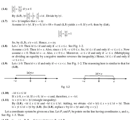
(1.8)
Let
c ≥
0. Then |
x
|
≤
c
if and only if
−c ≤
x ≤
c.
See Fig. 1-2.
Assume
x
≥
0. Then
|x| = x.
Also, since
c ≥
0,
−c ≤
0
≤
x
. So,
|x| ≤
c
if and only if
−c ≤
x ≤
c.
Now
assume
x
<
0. Then |
x
|
=
−x
. Also,
x
<
0
≤
c.
Moreover,
−x
≤
c
if and only if
−c ≤
x.
(Multiplying
or dividing an equality by a negative number reverses the inequality.) Hence, |
x
|
≤
c
if and only if
−c ≤
x ≤
c.
(1.9)
Let
c ≥
0. Then |
x
|
<
c
if and only if
−c < x < c.
See Fig. 1-2. The reasoning here is similar to that for
(1.8)
.
Fig. 1-2
(1.10)
−
|
x
|
≤
x
≤
|
x
|
If
x
≥
0,
x
=
|
x
|. If
x
<
0, |
x
|
=
−x
and, therefore,
x = −|x
|.
(1.11)
|x +
y| ≤
|x| +
|y|
(triangle inequality)
By
(
1.8
),
−
|
x
|
≤
x
≤
|
x
| and
−
|
y
|
≤
y ≤
|
y|.
Adding, we obtain
−
(|
x
|
+
|
y
|)
≤
x
+
y ≤
|
x
|
+
|y|.
Then
|
x
+
y| ≤
|x| +
|y|
by (
1.8
). [In (
1.8
), replace
c
by |
x
|
+
|y|
and
x
by
x +
y.
]
Let a coordinate system be given on a line. Let
P
1and
P
2be points on the line having coordinates
x
1and
x
2.
See Fig. 1-3. Then:
(1.12)
|
x
1−
x
2|
=
P
1P
2=
distance between
P
1and
P
2.
This is clear when 0
<
x
1< x
2and when
x
1<
x
2<
0. When
x
1<
0
<
x
2, and if we denote the origin
by
O,
then
P
1P
2=
P
1O
+
OP
2=
(
−x
1)
+
x
2=
x
2−
x
1=
|
x
2−
x
1|
=
|x
1− x
2|.
As a special case of (
1.12
), when
P
2is the origin (and
x
2=
0):
(1.13)
|
x
1|
=
distance between
P
1and the origin.
Fig. 1-3
Finite Intervals
Let
a
<
b.
The
open interval
(
a, b
)
is defined to be the set of all numbers between
a
and
b,
that is, the set of all
x
such
that
a
<
x
<
b.
We shall use the term
open interval
and the notation (
a, b
)
also for all the points between the
points with coordinates
a
and
b
on a line. Notice that the open interval (
a, b
)
does not contain the
endpoints
a
and
b.
See Fig. 1-4.
Fig. 1-4
By a
half-open interval
we mean an open interval (
a, b
)
together with one of its endpoints. There are two
such intervals: [
a, b
)
is the set of all
x
such that
a ≤
x < b,
and (
a, b
]
is the set of all
x
such that
a < x ≤
b.
Infinite Intervals
Let (
a, ∞
)
denote the set of all
x
such that
a < x.
Let [
a, ∞
)
denote the set of all
x
such that
a ≤ x.
Let (
−∞
,
b
)
denote the set of all
x
such that
x < b.
Let (
−∞
,
b
]
denote the set of all
x
such that
x ≤ b.
Inequalities
Any inequality, such as
2x −
3
>
0 or 5
<
3
x +
10
≤
16, determines an interval. To solve an inequality means
to determine the corresponding interval of numbers that satisfy the inequality.
EXAMPLE 1.1: Solve 2x − 3 > 0.
2
3
0
2
3
3 2
x
x
x
− >
>
>
(Adding 3)
(Dividing by 2)
Thus, the corresponding interval is
( , ).
3 2∞
EXAMPLE 1.2: Solve 5 < 3x + 10 ≤ 16.5 3 10 16
5 3 6
2 5 3
< + ≤ − < ≤ − < ≤
x x x
(Subtracting 10) (Diviiding by 3) Thus, the corresponding interval is (−5,
3 2]. EXAMPLE 1.3: Solve −2x + 3 < 7.
− + <
−
<
> −
−
2
3
7
2
4
2
x
x
x
(Subtracting 3)
(Dividing by
2))
(Recall that dividing by a negative number reverses an inequality.) Thus, the corresponding interval is (−2, ∞).
SOLVED PROBLEMS
1. Describe and diagram the following intervals, and write their interval notation, (a) −3 < x < 5; (b) 2 ≤ x ≤ 6; (c) −4 < x ≤ 0; (d) x > 5; (e) x ≤ 2; (f ) 3x − 4 ≤ 8; (g) 1 < 5 − 3x < 11.
(d) All numbers greater than 5; (5, ∞):
(
e
) All numbers less than or equal to 2; (−∞, 2]:(f) 3x − 4 ≤ 8 is equivalent to 3x ≤ 12 and, therefore, to x ≤ 4. Thus, we get (−∞, 4]:
(
g
) 1 5 3 114 3 6
2 4
3 < − < − < − < − < <
x x x
(Subtracting 5)
(Dividding by−3;note the reversal of inequalities) Thus, we obtain (−2, ):4
3
2. Describe and diagram the intervals determined by the following inequalities, (a) |x| < 2; (b) |x| > 3; (c) |x
−
3| < 1; (d) |x−
2| < d where d > 0; (e) |x + 2| ≤ 3; (f ) 0 < |x − 4| < d where d > 0.(a) By property (1.9), this is equivalent to −2 < x < 2, defining the open interval (−2, 2).
(
b
) By property (1.8), |x| ≤ 3 is equivalent to −3 ≤ x ≤ 3. Taking negations, |x| > 3 is equivalent to x < −3 or x > 3, which defines the union of the intervals (−∞, −3) and (3, ∞).(
c
) By property (1.12), this says that the distance between x and 3 is less than 1, which is equivalent to 2 < x < 4. This defines the open interval (2, 4).We can also note that |x − 3| < 1 is equivalent to −l < x − 3 < 1. Adding 3, we obtain 2 < x < 4.
(e) |x + 2| < 3 is equivalent to −3 < x + 2 < 3. Subtracting 2, we obtain −5 < x < 1, which defines the open interval (−5, 1):
(f) The inequality |x − 4| < d determines the interval 4 − d < x < 4 + d. The additional condition 0 < |x − 4| tells us that x ≠ 4. Thus, we get the union of the two intervals (4 − d, 4) and (4, 4 + d ). The result is called the deleted d-neighborhood of 4:
3. Describe and diagram the intervals determined by the following inequalities, (a) |5 − x| ≤ 3; (b) |2x − 3| < 5; (c) |1 − 4x| <1
2.
(a) Since |5 − x| = |x − 5|, we have |x − 5| ≤ 3, which is equivalent to −3 ≤ x − 5 ≤ 3. Adding 5, we get 2 ≤ x ≤ 8, which defines the closed interval [2, 8]:
(b) |2x − 3| < 5 is equivalent to −5 < 2x − 3 < 5. Adding 3, we have −2 < 2x < 8; then dividing by 2 yields −1 < x < 4, which defines the open interval (−1, 4):
(c) Since |1 − 4x| = |4x − 1|, we have |4x − 1| <1
2, which is equivalent to −12 < 4x − 1 < 12. Adding 1, we get 1
2 < 4x <32. Dividing by 4, we obtain 18< <x 83, which defines the open interval ( , )18 38 :
4. Solve the inequalities: (a) 18x − 3x2> 0; (b) (x + 3)(x − 2)(x − 4) < 0; (c) (x + l)2(x − 3) > 0, and diagram the solutions. (a) Set 18x − 3x2= 3x(6 − x) = 0, obtaining x = 0 and x = 6. We need to determine the sign of 18x − 3x2 on each
of the intervals x < 0, 0 < x < 6, and x > 6, to determine where 18x − 3x2> 0. Note that it is negative when x < 0 (since x is negative and 6 − x is positive). It becomes positive when we pass from left to right through 0 (since x changes sign but 6 − x remains positive), and it becomes negative when we pass through 6 (since x remains positive but 6 − x changes to negative). Hence, it is positive when and only when 0 < x < 6.
(b) The crucial points are x = −3, x = 2, and x = 4. Note that (x + 3)(x − 2)(x − 4) is negative for x < −3 (since each of the factors is negative) and that it changes sign when we pass through each of the crucial points. Hence, it is negative for x < −3 and for 2 < x < 4:
(c) Note that (x + 1) is always positive (except at x = −1, where it is 0). Hence (x + 1)2 (x − 3) > 0 when and only when x − 3 > 0, that is, for x > 3:
5. Solve |3x − 7| = 8.
By (1.3), |3x − 7| = 8 if and only if 3x − 7 =±8. Thus, we need to solve 3x − 7 = 8 and 3x − 7 = −8. Hence, we get x = 5 or x =− 1
Case 2: x + 3 < 0. Multiply by x + 3 to obtain 2x + 1 < 3x + 9. (Note that the inequality is reversed, since we multiplied by a negative number.) This yields −8 < x. Since x + 3 < 0, we have x < −3. Thus, the only solutions are −8 < x < −3.
7. Solve 2 3 5 x− < .
The given inequality is equivalent to −5 < 2 − 3 < 5. Add 3 to obtain −2 < 2/x < 8, and divide by 2 to get −1 < l/x < 4.
Case 1: x > 0. Multiply by x to get −x < 1 < 4x. Then x >1
4 and x > −1; these two inequalities are equivalent to the single inequality x >1
4.
Case 2: x < 0. Multiply by x to obtain −x > 1 > 4x. (Note that the inequalities have been reversed, since we multiplied by the negative number x.) Then x <1
4 and x < −1. These two inequalities are equivalent to x < −1. Thus, the solutions are x >1
4 or x < −1, the union of the two infinite intervals (14, •) and (−•, −1). 8. Solve |2x − 5| ≥ 3.
Let us first solve the negation |2x − 5| < 3. The latter is equivalent to −3 < 2x − 5 < 3. Add 5 to obtain 2 < 2x < 8, and divide by 2 to obtain 1 < x < 4. Since this is the solution of the negation, the original inequality has the solution x ≤ 1 or x ≥ 4.
9. Solve: x2< 3x + 10.
x2< 3x + 10
x2 − 3x − 10 < 0 (Subtract 3x + 10) (x − 5)(x + 2) < 0
The crucial numbers are −2 and 5. (x − 5)(x + 2) > 0 when x < −2 (since both x − 5 and x + 2 are negative); it becomes negative as we pass through −2 (since x + 2 changes sign); and then it becomes positive as we pass through 5 (since x − 5 changes sign). Thus, the solutions are − 2 < x < 5.
SUPPLEMENTARY PROBLEMS
10. Describe and diagram the set determined by each of the following conditions: (a) −5 < x < 0 (b) x ≤ 0
(c) −2 ≤ x < 3 (d) x ≥ 1 (e) |x | < 3 (f ) |x | ≥ 5 (g) |x − 2| <1
2 (h) |x − 3| > 1
(i) 0 < |x − 2| < 1 ( j) 0 < |x + 3| <1 4 (k) |x − 2| ≥ 1.
Ans. (e) −3 < x < 3; (f )x ≥ 5 orx ≤ −5; (g) 3
2 < x < 52; (h) x >−2 orx < −4; (i)x ≠ 2 and 1 < x < 3; ( j) −13
4 < x < −114; (k) x ≥3 orx ≤ 1
11. Describe and diagram the set determined by each of the following conditions: (a) |3x − 7| < 2
(b) |4x − l| ≥ 1 (c) x
(d) 3 2 4 x− ≤ (e) 2+1 >1
x (f ) 4 3 x < Ans. (a)5
3 < x < 3; (b)x ≥ 12orx ≤ 0; (c) −6 ≤ x ≤ 18; (d)x ≤ −23orx ≥ 12;(e)x > 0 orx < −1 or −13 < x < 0; (f )x > 4
3orx < −43
12. Describe and diagram the set determined by each of the following conditions: (a) x(x − 5) < 0
(b) (x − 2)(x − 6) > 0 (c) (x + l)(x − 2) < 0 (d) x(x − 2)(x + 3) > 0 (e) (x + 2)(x + 3)(x + 4) < 0 (f ) (x − 1)(x + 1)(x − 2)(x + 3) > 0 (g) (x − l)2(x + 4) > 0
(h) (x − 3)(x + 5)(x − 4)2< 0 (i) (x − 2)3> 0
( j) (x + 1)3< 0 (k) (x − 2)3(x + l) < 0 (l) (x − 1)3 (x + 1)4 < 0 (m) (3x − l)(2x + 3) > 0 (n) (x − 4) (2x − 3) < 0
Ans. (a) 0 < x < 5; (b)x > 6 orx < 2; (c) −1 < x < 2; (d)x > 2 or −3 < x < 0; (e) −3 < x < −2 orx < −4; (f )x > 2 or − 1 < x < 1 orx < −3; (g) x > −4 andx ≠ 1; (h) −5 < x < 3; (i)x > 2; ( j) x < −1; (k) −1 < x < 2; (l)x < 1 andx ≠ −1; (m)x > 1
3orx < −32;(n)32 < x < 4 13. Describe and diagram the set determined by each of the following conditions:
(a) x2< 4 (b) x2≥ 9 (c) (x − 2)2≤ 16 (d) (2x + 1)2 > 1 (e) x2+ 3x − 4 > 0 (f ) x2+ 6x + 8 ≤ 0 (g) x2< 5x + 14 (h) 2x2> x + 6 (i) 6x2+ 13x < 5 ( j) x3+ 3x2> 10x
Ans. (a) −2 < x < 2; (b) x ≥ 3 orx ≤ −3; (c) −2 ≤ x ≤ 6; (d)x > 0 orx < −1; (e)x > 1 orx < −4; (f ) −4 ≤ x ≤ −2; (g) −2 < x < 7; (h)x > 2 orx < − 3
2;(i) − < <52 x 31; ( j) −5 < x < 0 orx > 2 14. Solve: (a) −4 < 2 − x < 7 (b) 2x 1 3
x − <
(c) x
x+ <2 1 (d) 3 1
2 3 3
x x −
+ > (e) 2xx 1 2
− > (f) x
x+2 ≤2 Ans. (a) −5< x < 6; (b) x > 0 orx < −1; (c)x > −2; (d) − < <10
(d) |x + 1| = |x + 2| (e) |x + 1| = 3x − 1 (f ) |x + 1| < |3x − 1| (g) |3x − 4| ≥ |2x + 1|
Ans. (a)x = 2 orx = 1
2;(b)x = −4 orx = −8; (c)x = 5 orx = 53;(d)x = −32; (e)x = 1; (f ) x >1 orx < 0; (g) x ≥5 orx ≤ 3
5
16. Prove: (a) |x2| = |x|2;
(b) |xn| = |x|n for every integer n; (c) |x| = x2;
(d) |x − y| ≤ |x| + |y|; (e) |x − y| ≥ ||x| − |y||
9
Rectangular Coordinate
Systems
Coordinate Axes
In any plane
ᏼ
, choose a pair of perpendicular lines. Let one of the lines be horizontal. Then the other line
must be vertical. The horizontal line is called the
x
axis
, and the vertical line the
y axis
. (See Fig. 2-1.)
Fig. 2-1
Now choose linear coordinate systems on the
x
axis and the
y
axis satisfying the following conditions:
The origin for each coordinate system is the point
O
at which the axes intersect. The
x
axis is directed from
left to right, and the
y
axis from bottom to top. The part of the
x
axis with positive coordinates is called the
positive x axis
, and the part of the
y
axis with positive coordinates is called the
positive y
axis
.
We shall establish a correspondence between the points of the plane
ᏼ
and pairs of real numbers.
Coordinates
Consider any point
P
of the plane (Fig. 2-1). The vertical line through
P
intersects the
x
axis at a unique
point; let
a
be the coordinate of this point on the
x
axis. The number
a
is called the
x coordinate
of
P
(or the
abscissa
of
P
). The horizontal line through
P
intersects the
y
axis at a unique point; let
b
be the coordinate
of this point on the
y
axis. The number
b
is called the
y coordinate
of
P
(or the
ordinate
of
P
). In this way,
every point
P
has a unique pair (
a
,
b
) of real numbers associated with it. Conversely, every pair (
a
,
b
) of real
numbers is associated with a unique point in the plane.
Fig. 2-2
EXAMPLE 2.1: In the coordinate system of Fig. 2-3, to find the point having coordinates (2, 3), start at the origin, move two units to the right, and then three units upward.
Fig. 2-3
To find the point with coordinates (−4, 2), start at the origin, move four units to the left, and then two units upward. To find the point with coordinates (−3, −1), start at the origin, move three units to the left, and then one unit downward. The order of these moves is not important. Hence, for example, the point (2, 3) can also be reached by starting at the origin, moving three units upward, and then two units to the right.
Quadrants
Assume that a coordinate system has been established in the plane
ᏼ
. Then the whole plane
ᏼ
, with the
Quadrant
II consists of all points with negative
x
coordinate and positive
y
coordinate.
Quadrants
III and IV
are also shown in Fig. 2-4.
Fig. 2-4
The points on the
x
axis have coordinates of the form (
a
, 0). The
y
axis consists of the points with
coor-dinates of the form (0,
b
).
Given a coordinate system, it is customary to refer to the point with coordinates (
a
,
b
) as “the point
(
a
,
b
).” For example, one might say, “The point (0, 1) lies on the
y
axis.”
The Distance Formula
The distance
P
1P
2between poinits
P
1and
P
2with coordinates (
x
1,
y
1) and (
x
2,
y
2) in a given coordinate system
(see Fig. 2-5) is given by the following distance formula:
P P
1 2x
1x
2y
y
2
1 2
2
=
(
−
)
+
(
−
)
(2.1)Fig. 2-5
To see this, let
R
be the point where the vertical line through
P
2intersects the horizontal line through
P
1. The
x
coordinate of
R
is
x
2, the same as that of
P
2. The
y
coordinate of
R
is
y
1, the same as that of
P
1. By the
Pythago-rean theorem, (
P P
1 2)
(
P R
)
(
P R
)
2 1
2 2
2
=
+
. If
A
1and
A
2are the projections of
P
1and
P
2on the
x
axis, the segments
P
1R
and
A
1A
2are opposite sides of a rectangle, so that
P R
1=
A A
1 2. But
A A
1 2=
|
x
1−
x
2| by property (
1.12
).
So,
P R
x
x
1
=
|
1−
2| . Similarly,
P R
2=
|
y
1−
y
2|. Hence, (
P P
1 2)
x
x
y
y
(
x
x
)
(
y
y
)
21 2
2
1 2 2
1 2
2
1 2
2
(a) The distance between (2, 5) and (7, 17) is
(2 7− )2+ −(5 17)2 = (−5)2+ −( 12)2 = 25 144+ = 169=13 (b) The distance between (1, 4) and (5, 2) is
(1 5− )2+(4−2)2 = (−4)2+( )22 = 16 4+ = 20= 4 5=2 5
The Midpoint Formulas
The point
M
(
x
,
y
) that is the midpoint of the segment connecting the points
P
1(
x
1,
y
1) and
P
2(
x
2,
y
2) has the
coordinates
x
=
x
1+
x
2y
=
y
1+
y
22
2
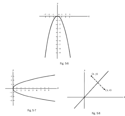
(2.2)Thus, the coordinates of the midpoints are the averages of the coordinates of the endpoints. See Fig. 2-6.
Fig. 2-6
To see this, let
A
,
B, C
be the projections of
P
1,
M, P
2on the
x
axis. The
x
coordinates of
A, B, C
are
x
1,
x
,
x
2. Since the lines
P
1A, MB
, and
P
2C
are parallel, the ratios
P M MP
1/
2and
AB BC
/
are equal. Since
P M
1=
MP
2,
AB
=
BC
. Since
AB
= −
x
x
1and
BC
=
x
2−
x
,
x
x
x
x
x
x
x
x
x
x
−
=
−
=
+
=
+
1 2
1 2
1 2
2
2
(The same equation holds when
P
2is to the left of
P
1, in which case
AB
= −
x
1x
and
BC
= −
x
x
2.)
Similarly,
y
=
(
y
1+
y
2)
/
2.
EXAMPLES:
(a) The midpoint of the segment connecting (2, 9) and (4, 3) is 2 4 2
9 3
2 3 6
+ + ⎞
⎠⎟ = ⎛
⎝⎜ , ( , ).
(b) The point halfway between (−5, 1) and (1, 4) is ⎛− + +
⎝⎜ ⎞⎠⎟ = −
(
)
5 12 1 4
2 2
5 2
Proofs of Geometric Theorems
Proofs of geometric theorems can often be given more easily by use of coordinates than by deductions from
axioms and previously derived theorems. Proofs by means of coordinates are called
analytic
, in contrast to
so-called
synthetic
proofs from axioms.
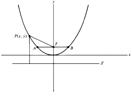
EXAMPLE 2.2: Let us prove analytically that the segment joining the midpoints of two sides of a triangle is one-half the length of the third side. Construct a coordinate system so that the third side AB lies on the positive x axis, A is the origin, and the third vertex C lies above the x axis, as in Fig. 2-7.
Fig. 2-7
Let b be the x coordinate of B. (In other words, let b=AB.) Let C have coordinates (u, v). Let M
1 and M2 be the midpoints of sides AC and BC, respectively. By the midpoint formulas (2.2), the coordinates of M1 are
(
u2 2, v)
, and the coordinates of M2 are
(
u+b)
2 , 2
v
. By the distance formula (2.1),
M M1 2 u u b b
2 2 2
2 2 2 2 2
= ⎛⎝⎜ − + ⎞⎠⎟ +⎛⎝⎜v −v⎞⎠⎟ = ⎝⎜⎛ ⎞⎠⎟ =bb
2 which is half the length of side AB.
SOLVED PROBLEMS
1. Show that the distance between a point P(x, y) and the origin is x2+y2.
Since the origin has coordinates (0, 0), the distance formula yields (x−0)2+ −(y 0)2 = x2+y2. 2. Is the triangle with vertices A(1, 5), B(4, 2), and C(5, 6) isosceles?
AB AC
= − + − = − + = + =
= −
( ) ( ) ( ) ( )
( )
1 4 5 2 3 3 9 9 18
1 5
2 2 2 2
2++ − = − + − = + =
= − + −
( ) ( ) ( )
( ) ( )
5 6 4 1 16 1 17
4 5 2 6
2 2 2
2
BC 22 = (−1)2+ −( 4)2 = 1 16+ = 17 Since AC=BC, the triangle is isosceles.
2 5 (
= −
BC ))2+(3 10− )2 = (−3)2+ −( 7)2 = 9+49= 58
Since AC2=AB2+BC2, the converse of the Pythagorean theorem tells us that Δ ABC is a right triangle, with right angle at B; in fact, since AB=BC, Δ ABC is an isosceles right triangle.
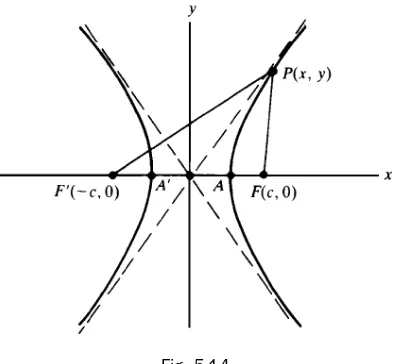
4. Prove analytically that, if the medians to two sides of a triangle are equal, then those sides are equal. (Recall that a median of a triangle is a line segment joining a vertex to the midpoint of the opposite side.)
In Δ ABC, let M1 and M2 be the midpoints of sides AC and BC, respectively. Construct a coordinate system so that A is the origin, B lies on the positive x axis, and C lies above the x axis (see Fig. 2-8). Assume that
AM2=BM1. We must prove that AC=BC. Let b be the x coordinate of B, and let C have coordinates (u, v).
Then, by the midpoint formulas, M1 has coordinates u 2 2,
v
(
)
, and M2 has coordinates(
u+b)
2 , 2v .
Hence,
Fig. 2-8
AM2 u b
2 2
2 2
= ⎛⎝⎜ + ⎞⎠⎟ +⎛⎝⎜v⎞⎠⎟
and BM1 u b
2 2
2 2
= ⎛⎝⎜ − ⎞⎠⎟ +⎛⎝⎜v⎞⎠⎟
Since AM2=BM1,
u b u
b +
⎛
⎝⎜ 2 ⎠⎟ +⎞ ⎛⎝⎜2⎞⎠⎟ =⎛⎝⎜2− ⎞⎠⎟ +⎝⎜⎛2⎞⎠⎟
2 2 2 2
v v
==⎛⎝⎜u−22b⎞⎠⎟ +⎛⎝⎜2⎞⎠⎟
2 2
v
Hence, (u+b) + =(u− b) + 2
2 2 2
4 4
2
4 4
v v and, therefore, (u + b)2 = (u − 2b)2. So, u + b = ±(u − 2b). If u + b = u − 2b, then b = −2b, and therefore, b = 0, which is impossible, since A ≠ B. Hence, u + b = − (u − 2b) = −u + 2b, whence 2u = b. Now BC= (u−b)2+v2 = (u−2u)2+v2 = (−u)2+v2 = u2+v2, and AC= u2+v2. Thus, AC=BC.
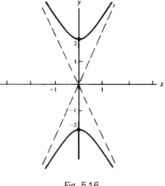
5. Find the coordinates (x, y) of the point Q on the line segment joining P1(1, 2) and P2(6, 7), such that Q divides the segment in the ratio 2 : 3, that is, such that P Q QP1 2 2
3
/ = .
Let the projections of P1, Q, and P2 on the x axis be A1, Q′, and A2, with x coordinates 1, x, and 6, respectively (see Fig. 2-9). Now A Q Q A PQ QP
1 2 1 2
2 3
segments are in proportion.) But A Q1 ′ = −x 1, and Q A′ = −2 6 x. So x x − − =1 6
2
3, and cross-multiplying yields 3x − 3 = 12 − 2x. Hence 5x = 15, whence x = 3. By similar reasoning, y
y − − =2
7 23, from which it follows that y = 4.
Fig. 2-9
SUPPLEMENTARY PROBLEMS
6. In Fig. 2-10, find the coordinates of points A, B, C, D, E, and F.
Fig. 2-10
Ans. (A) = (−2, 1); (B) = (0, −1); (C) = (1, 3); (D) = (−4, −2); (E) = (4, 4); (F ) = (7, 2).
7. Draw a coordinate system and show the points having the following coordinates: (2, −3), (3, 3), (−1, 1), (2, −2), (0, 3), (3, 0), (−2, 3).
8. Find the distances between the following pairs of points:
(a) (3, 4) and (3, 6) (b) (2, 5) and (2, −2) (c) (3, 1) and (2, 1) (d) (2, 3) and (5, 7) (e) (−2, 4) and (3, 0) (f )
(
−2 1)
2
, and (4, −1) Ans. (a) 2; (b) 7; (c) 1; (d) 5; (e) 41; (f) 3
2 17
11. If the points (2, 4) and (−1, 3) are the opposite vertices of a rectangle whose sides are parallel to the coordinate axes (that is, the x and y axes), find the other two vertices.
Ans. (−1, 4) and (2, 3)
12. Determine whether the following triples of points are the vertices of an isosceles triangle: (a) (4, 3), (1, 4), (3, 10); (b) (−1, 1), (3, 3), (1, −1); (c) (2, 4), (5, 2), (6, 5).
Ans. (a) no; (b) yes; (c) no
13. Determine whether the following triples of points are the vertices of a right triangle. For those that are, find the area of the right triangle: (a) (10, 6), (3, 3), (6, −4); (b) (3, 1), (1, −2), (−3, −1); (c) (5, −2), (0, 3), (2, 4).
Ans. (a) yes, area = 29; (b) no; (c) yes,
area
=
15 214. Find the perimeter of the triangle with vertices A(4, 9), B(−3, 2), and C(8, −5). Ans. 7 2+ 170+2 53
15. Find the value or values of y for which (6, y) is equidistant from (4, 2) and (9, 7). Ans. 5
16. Find the midpoints of the line segments with the following endpoints: (a) (2, −3) and (7, 4); (b) 5
(
3,2)
and (4, 1); (c) ( 3 0 and (1, 4)., )Ans. (a)
(
92, 12)
; (b)(
176, 32)
; (c) ⎛1+2 3 2 ⎝⎜⎞ ⎠⎟ ,
17. Find the point (x, y) such that (2, 4) is the midpoint of the line segment connecting (x, y) and (1, 5). Ans. (3, 3)
18. Determine the point that is equidistant from the points A(−1, 7), B(6, 6), and C(5, −1). Ans. 52
25,15350
(
)
19. Prove analytically that the midpoint of the hypotenuse of a right triangle is equidistant from the three vertices.
20. Show analytically that the sum of the squares of the distance of any point P from two opposite vertices of a rectangle is equal to the sum of the squares of its distances from the other two vertices.
22. Prove analytically that the sum of the squares of the medians of a triangle is equal to three-fourths the sum of the squares of the sides.
23. Prove analytically that the line segments joining the midpoints of opposite sides of a quadrilateral bisect each other.
24. Prove that the coordinates (x, y) of the point Q that divides the line segments from P1(x1, y1) to P2(x2, y2) in the ratio r1 : r2 are determined by the formulas
x r x r x
r r y
r y r y r r = 1 2++ 2 1 = ++
1 2
1 2 2 1 1 2 and
(Hint: Use the reasoning of Problem 5.)
25. Find the coordinates of the point Q on the segment P1P2 such that PQ QP1 2 2 7
/ = , if (a) P1 = (0, 0), P2 = (7, 9); (b) P1 = (−1, 0), P2 = (0, 7); (c) P1 = (−7, −2), P2 = (2, 7); (d) P1 = (1, 3), P2 = (4, 2).
Ans. (a) 14 9,2
(
)
; (b)(
−7)
18
The Steepness of a Line
The steepness of a line is measured by a number called the
slope
of the line. Let
ᏸ
be any line, and let
P
1
(
x
1,
y
1)
and
P
2(
x
2,
y
2) be two points of
ᏸ
. The slope of
ᏸ
is defined to be the number
m
y
y
x
x
=
2−
−
12 1
. The slope is the
ratio of a change in the
y
coordinate to the corresponding change in the
x
coordinate. (See Fig. 3-1.)
Fig. 3-1
For the definition of the slope to make sense, it is necessary to check that the number
m
is independent
of the choice of the points
P
1and
P
2. If we choose another pair
P
3(
x
3,
y
3) and
P
4(
x
4,
y
4), the same value of
m
must result. In Fig. 3-2, triangle
P
3P
4T
is similar to triangle
P
1P
2Q
. Hence,
QP
PQ
TP
P T
2 14 3
=
ory
y
x
x
y
y
x
x
2 1
2 1
4 3
4 3
−
−
=
−
−
Therefore,
P
1and
P
2determine the same slope as
P
3and
P
4.
EXAMPLE 3.1: The slope of the line joining the points (1, 2) and (4, 6) in Fig. 3-3 is 64 1−− =2 43. Hence, as a point on the line moves 3 units to the right, it moves 4 units upwards. Moreover, the slope is not affected by the order in which the points are given: 2 6
1 4− =− −− =43 43. In general,
y y
x x
y y
x x
2 1 2 1
1 2 1 2 −
− = −− .
The Sign of the Slope
The sign of the slope has significance. Consider, for example, a line
ᏸ
that moves upward as it moves to the
right, as in Fig. 3-4(
a
). Since
y
2>
y
1and
x
2>
x
1, we have
m
y
y
x
x
=
2−
−
1>
2 1
0.
The slope of
ᏸ
is positive
.
Now consider a line
ᏸ
that moves downward as it moves to the right, as in Fig. 3-4(
b
). Here
y
2
<
y
1while
x
2>
x
1; hence,
m
y
y
x
x
=
2−
−
1<
2 1
Fig. 3-2 Fig. 3-3
Now let the line
ᏸ
be horizontal, as in Fig. 3-4(
c
). Here
y
1
=
y
2, so that
y
2−
y
1=
0. In addition,
x
2−
x
1≠
0.
Hence,
m
x
x
=
−
0
=
0
2 1
.
The slope of
ᏸ
is zero
.
Line
ᏸ
is vertical in Fig. 3-4(
d
), where we see that
y
2
−
y
1>
0 while
x
2−
x
1=
0. Thus, the expression
y
y
x
x
2 1
2 1
−
−
is undefined.
The slope is not defined for a vertical line
ᏸ
. (Sometimes we describe this situation by
saying that the slope of
ᏸ
is “infinite.”)
Fig. 3-4
Slope and Steepness
Consider any line
ᏸ
with positive slope, passing through a point
P
1
(
x
1,
y
1); such a line is shown in Fig. 3-5.
Choose the point
P
2(
x
2,
y
2) on
ᏸ
such that
x
2
−
x
1=
1. Then the slope
m
of
ᏸ
is equal to the distance
AP
2.
As the steepness of the line increases,
AP
2increases without limit, as shown in Fig. 3-6(
a
). Thus, the slope
of
ᏸ
increases without bound from 0 (when
ᏸ
is horizontal) to
+∞
(when the line is vertical). By a similar
Fig. 3-5
Fig. 3-6
Equations of Lines
Let
ᏸ
be a line that passes through a point
P
1
(
x
1,
y
1) and has slope
m
, as in Fig. 3-7(
a
). For any other point
P
(
x
,
y
) on the line, the slope
m
is, by definition, the ratio of
y
−
y
1to
x
−
x
1. Thus, for any point (
x
,
y
) on
ᏸ
,
m
y
y
x
x
=
−
−
11 (3.1)