TESIS SS09-2304
PRACTICAL METHODS VALIDATION FOR VARIABLES
SELECTION IN THE HIGH DIMENSION DATA:
APPLICATION FOR THREE METABOLOMICS DATASETS
ACHMAD CHOIRUDDIN NRP 1312 201 905
PEMBIMBING
Jean-Charles MARTIN Mat t hieu MAILLOT Fl orent VIEUX Cécil e CAPPONI
PROGRAM MAGISTER JURUSAN STATISTIKA
FAKULTAS MATEMATIKA DAN ILMU PENGETAHUAN ALAM INSTITUT TEKNOLOGI SEPULUH NOPEMBER
THESIS SS09-2304
PRACTICAL METHODS VALIDATION FOR VARIABLES
SELECTION IN THE HIGH DIMENSION DATA:
APPLICATION FOR THREE METABOLOMICS DATASETS
ACHMAD CHOIRUDDIN NRP 1312 201 905
SUPERVISORS
Jean-Charles MARTIN Mat t hieu MAILLOT Fl orent VIEUX Cécil e CAPPONI
MAGISTER PROGRAM
DEPARTMENT OF STATISTICS
FACULTY OF MATHEMATICS AND NATURAL SCIENCES INSTITUT TEKNOLOGI SEPULUH NOPEMBER
ABSTRACT
Background: Variable selection on high throughput metabolomics data are becoming inevitable to select relevant information since they often imply a high degree of multicolinearity, and, as a result, lead to severely ill conditioned problems. Both in supervised classification framework and machine learning algorithms, one solution is to reduce their data dimensionality either by performing features selection, or by introducing artificial variables in order to enhance the generalization performance of a given algorithm as well as to gain some insight about the concept to learned.
Objective: The main objective of this study is to select a set of features from thousands of variables in dataset. We divide this objective into two sides: (1) To identify small sets of features (fewer than 15 features) that could be used for diagnostic purpose in clinical practice, called low-level analysis and (2) We do the identification to a larger set of features (around 50-100 features), called middle-level analysis; this involves obtaining a set of variables that are related to the outcome of interest. Besides that, we would like to compare the performances of several proposed techniques in feature selection procedure for Metabolomics study.
Method: This study is facilitated by four proposed techniques, which are two machine learning techniques (i.e., RSVM and RFFS) and two supervised classification techniques (i.e., PLS-DA VIP and sPLS-DA), to classify our three datasets, i.e., human urines, rat’s urines, and rat’s plasma datasets, which contains two classes sample each dataset.
Results: RSVM-LOO always leads the accuracy performance compare to the other two cross-validation methods, i.e., bootstrap and N-fold. However, this RSVM results is not much better since RFFS could achieve the higher accuracy performance. Another side, PLS-DA and sPLS-DA could reach a good performance either for variability explanation or predictive ability. In biological sense, RFFS and PLS-DA VIP show their performance by finding the more common selected features than RSVM and sPLS-DA compare to previous metabolomics study. This is also confirmed in the statistical comparison that RFFS and PLS-DA could lead the similarity percentage of selected features. Furthermore, RFFS and PLS-DA VIP have their better performance since they could select three metabolites of five confirmed metabolites from previous metabolomics study which couldn’t be achieved by RSVM and sPLS-DA.
Conclusion: RFFS seems to become the most appropriate techniques in features selection study, particularly in low-level analysis when having small sets features is often desirable. Both PLS-DA VIP and sPLS-PLS-DA lead to a good performance either for variability explanation or predictive ability, but PLS-DA VIP is slightly better in term of biological insight. Besides it is only limited for two class problem, RSVM unfortunately couldn’t achieve a quite good performance both in statistical and biological interpretation.
ACKNOWLEDGMENTS
Conducting a research with some experts in mostly metabolomics is really my first experience. Although I did take big efforts, I really enjoy doing this project in the sense that I could learn many new things. However, it would not have been possible without the kind support and help of many individuals and organizations. I would like to extend my sincere thanks to all of them.
My first thanks go to my supervisors for their continuous support and their precious feedback in conducting this project. I am highly indebted to Jean-Charles MARTIN for his kind to allow me carrying out a six-month internship in UMR NORT, getting involved in his research project team could deepen my analysis skill and broaden my knowledge. In addition, his experience as an expert taught me many things, not only on the project implementation, but also being a professional researcher. I would like to express my deep gratitude to Matthieu MAILLOT and
Florent VIEUX for their guidance and constant supervision as well as for providing necessary information regarding the project. I also particularly appreciated for their support and motivation both in completing the project and being my new family. Advice given by my university advisor,
Cécile CAPPONI, has been a great help in understanding several concepts I learned.
My thanks and appreciations also go to my colleagues in the laboratory of UMR NORT in developing the project and people who have willingly helped me out with their abilities.
I would further like to thank all the persons who helped me during my stay in the Department of Applied Mathematics in Social Sciences: a very kind people, Nicolas PECH, head of department, who gave a lot of time, energy, and motivation to keep me stand up until the end of this Master program, my great lecturers: Marie-christine ROUBAUD, Thomas WILLER, Laurence REBOUL, Sébastian OLIVEAU, Christine CAMPIONI, Rebecca McKenna, and
Richard LALOU who inspired me a lot, Fabienne PICOLET for her useful help in administration purpose, and for all my classmates : Dian, Julien, Lylia, Mahmoud, Armand, Alpha, Sofiane, and Youssoupha, we are truly the rainbow troops.
I would also like to acknowledge the Ministry of Education and Culture Republic of Indonesia, ITS Postgraduate program, and Ministry of Foreign Affair of France for the financial support.
TABLE OF CONTENT
ACKNOWLEDGMENTS ...ii
TABLE OF CONTENT ...iii
ABSTRACT ...iv
CHAPTER 1 PRESENTATION OF UMR NORT ...1
CHAPTER 2 INTRODUCTION ...3
2.1 Background ...3
2.2 Objective ...5
CHAPTER 3 LITERATURE REVIEW ...6
3.1 Support Vector Machine ...6
3.1.1. Recursive SVM ...7
3.1.2. Ranking the Features according to Their Contribution...8
3.1.3. Assessing the Performance of Feature Selection ...8
3.1.4. Recursive Classification and Feature Selection ...9
3.2 Random Forest ...11
3.2.1. Feature Selection Using Random Forest...12
3.2.2. Estimation of Error Rates in Feature Selection...12
3.3 Partial Least Squares Discriminant Analysis (PLS-DA) ...13
3.3.1. Feature Selection based on Variable Importance in the Projection ...14
3.3.2. Sparse PLSDA (sPLS-DA) ...15
CHAPTER 4 METHOD OF ANALYSIS ...17
4.1 Presentation of Datasets ...17
4.2 Statistical Analysis ...17
4.2.1 Pre-Processing Data ...17
4.2.2 R-Programming...18
4.2.3 Interpretation ...19
CHAPTER 5 ANALYSIS RESULTS ...20
5.1 Analysis Using R-SVM ...20
5.2 Analysis Using Random Forest for Feature Selection (RFFS) ...26
5.3 PLS-DA Feature Selection based on VIP ...28
5.4 Sparse PLS-DA (sPLS-DA) ...31
5.5 Methods Comparison ...34
5.6 Biological Interpretation ...38
CHAPTER 6 CONCLUSION AND PERSPECTIVE ...41
6.1 Conclusion ...41
6.2 Perspective ...42
REFERENCES ...43
1
CHAPTER 1
PRESENTATION OF UMR NORT
UMR NORT (Nutrition, Obésité et Risque Thrombotique) had many complementary expertise in the field of nutrition and metabolic diseases at the Faculty of Medicine in Timone, University of Aix-Marseille.
2 Two key complementary themes developed are: (1) digestion, bioavailability of lipophilic micro constituent and postprandial lipids metabolism, and (2) nutrition and vascular and thrombotic diseases. They combined both descriptive and mechanistic approaches using various and complementary methodologies ranging from molecular and cell biology to clinical studies.
3
CHAPTER 2
INTRODUCTION
Metabolomics is an emerging field providing insight into physiological processes. There have been a lot of metabolomics studies, and it is becoming more and more developed. In this part, we would like to describe the background overview of our metabolomics study, including background of our study and our study objectives.
2.1
Background
Metabolomics can be defined as the field of science that deals with the measurement of metabolites in an organism for the study of the physiological processes and their reaction to various stimuli such as infection, disease, or drug use (Nicholson, Lindon, & Holmes, 1999). It is an effective tool to investigate disease diagnosis in metabolite concentration in various biofluids.
Metabolomics allows analyzing hundreds of metabolites in a given biological sample. When applied to urine or plasma samples, it allows differentiating individual phenotypes better than with conventional clinical endpoints or with small sets of metabolites. It also allows exploring the metabolic effects of a nutrient in a more global way. In the field of nutrition, metabolomics has been used to characterize the effects of both a deficiency or a supplementation of different nutrients, and to compare the metabolic effects of closely related foods such as whole-grain or refined wheat flours (Scalbert, et al., 2009).
There have been several metabolomics studies which have been carried out, such as Kind, Tolstikov, Fiehn, & Weiss (2007) who did a research of urinary metabolomics approach for identifying kidney cancer, Gu, et al., (2007) who tested the effect of diet on metabolites using rat urine samples, and many others (Scalbert, et al., 2009; Suhre, et al., 2010; Dai, et al., 2010; and Grison, et al., 2013).
4 As these high throughput data are characterized by thousands of variables and small number of samples, they often imply a high degree of multicolinearity, and, as a result, lead to severely ill conditioned problems (Lê Cao, Boitard, & Besse, 2011). If directly working in this high dimensional space with limited samples, most conventional pattern recognition algorithms may not work well (Zhang & Wong, 2001). Some algorithms may not be able to achieve a solution when the number of sample is less than the dimensionality. For others that can achieve a solution, it may not be able to work well on samples other than that used for training.
Both in supervised classification framework and machine learning algorithms, one solution is to reduce the dimensionality of the data either by performing features selection, or by introducing artificial variables (i.e., latent variables) that summarize most of information. The purpose of the features or variables selection is to eliminate irrelevant variables to enhance the generalization performance of a given algorithm (Rakotomamonjy, 2003) as well as to gain some insight about the concept to be learned (Diaz-Uriarte & Andres, 2006). The technique of introducing artificial variables that summarize most of information, such as Partial Least Squares (PLS), has an objective to overcome the problem of high multicolinearity (Pérez-Enciso & Tenenhaus, 2003). Other advantages of feature selection and introducing artificial variables include cost reduction of data gathering and storage, and also on computational speedup.
Several features selection studies have been carried out. Golub, et al. (1999) defined a metric to evaluate the correlation of a feature with a classification scheme, thus determining whether the feature is relevant or not. Obviously, this kind of strategy does not take possible unless it can be proven that the features are statistically independent each other. Zhang & Wong (2001) proposed features selection algorithms named Recursive Support Vector Machines (R-SVM) based on the features contribution built by their weights and class means difference, while Guyon, Weston, Barnhill, & Vapnik (2002) proposed Support Vector Machine – Recursive Features Elimination (SVM-RFE) built by their weights in the SVM classifiers. In 2006, Zhang, et al., compared R-SVM and R-SVM-RFE and they concluded that R-R-SVM and R-SVM-RFE cross-validation prediction performances were nearly the same, but R-SVM was more robust to noise and outliers in discovering informative features and therefore had better accuracy on independent test data.
5 sparse PLS-DA (or sPLS-DA), which was a natural extension to the sPLS proposed by Lê Cao, Rossouw, Robert-Granié, & Besse (2008).
In this study, we will focus on the four methods proposed above (R-SVM, RFFS, PLSDA-VIP, and sPLS-DA) to analyze metabolomics data. It is important to identify the discriminating features that cause the categorization to enable an in-depth understanding of the system that generated the data. This can be achieved through feature selection, which involves identifying the optimum subset of the variables in data set that gives the best separation (Mahadevan, Shah, Marrie, & Slupsky, 2008).
2.2
Objective
Selection of relevant variables for sample classification is a common task in most features expression studies, including this study. When there are much larger features than the number of sample(s), this problem may undermine the success of classification techniques that is strongly affected by data quality: redundant, noisy, and unreliable information as well as a confusing selection of relevant variables. Because of that, our interest objectives in this study are as follows.
1. To identify small sets of features that could be used for diagnostic purpose in clinical practice; this involves obtaining the smallest possible set of variables that can still achieve good predictive performance. In this point, our purpose is to select the most relevant variables that contribute maximally in the classification (we define to choose under 15 features).
2. Beside the stringency depicted above to focus on the least number of variables enabling the best classification, our other purpose is to select a much wider set of variables (around 50-100 features) that detailed the outcome to be explained. This could provide a mechanistic view of the biological outcome to be described.
6
CHAPTER 3
LITERATURE REVIEW
In this part, we explain the statistical techniques used in this study. As mentioned in Chapter 2, headline of this study is to select a set of features from thousands of variables in dataset. Besides that, we would like to compare the performances of several proposed techniques in feature selection procedure for Metabolomics study. We consider three technique rules, which are Support Vector Machine (SVM), Random Forest (RF), and Partial Least Square Discriminant Analysis (PLS-DA). For feature selection, we will compare four techniques based on three rules mentioned. They are Recursive Support Vector Machine, Random Forest for Feature Selection, PLS-DA Feature Selection based on Variable Importance in the Projection, and Sparse PLS-DA.
3.1
Support Vector Machine
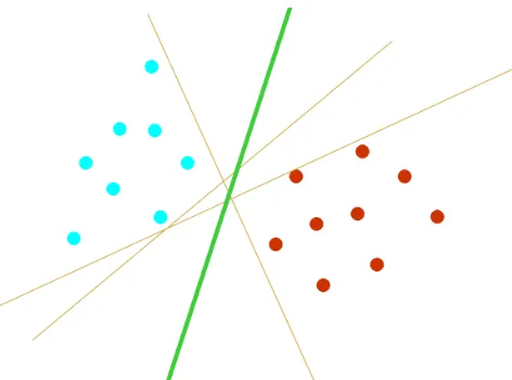
The basic principle of support vector machine classifier is a binary classifier algorithm that looks for an optimal hyper plane as a decision function in a high-dimensional space. The foundations of SVM have been developed by Cortes & Vapnik (1995) and are gaining popularity due to many attractive features, and promising empirical performance. In this problem, the goal is to separate the two classes by a function which is induced from available examples. The goal is to produce a classifier that will work well on unseen examples, i.e., it generalizes well. Consider the example in Figure 3.1. Here there are many possible linear classifiers that can separate the data, but there is only one that maximizes the margin (maximizes the distance between it and the nearest data point of each class). This linear classifier is termed the optimal separating hyper plane. Intuitively, we would expect this boundary to generalize well as opposed to the other possible boundaries.
7 SVM has been developed for multiclass purpose and even for regression problem. SVM techniques both in classification and regression purpose have been explained by Gunn (1998). In this study, we will focus on SVM for binary classification. The key idea of SVM is on generalization; where a classifier needs not only to work well on the training samples, but also work equally well on previously unseen samples.
Consider one has a training data set {𝒙𝑘,𝑦𝑘}∈ ℝ𝑛× {−1,1} where 𝒙𝑘are the training examples and 𝑦𝑘are the class labels. The method consists in first mapping x into a high dimensional space via a function𝚽, then computing a decision function of the form:
𝑓(𝒙) =〈𝒘,𝚽(𝒙)〉+𝑏
by maximizing the distance between the set of points 𝚽(𝒙) to the hyperplane parameterized by (𝒘,𝑏) while being consistent on the training set. The set of vectors is said to be optimally separated by the hyper plane if it is separated without error and the distance among the closest vectors to the hyper plane is maximal. The class label of x is obtained by considering the sign of𝑓(𝒙). For the SVM classifier with misclassified examples being quadratically penalized, this optimization problem can be written as:
min which is trade off between the training accuracy and prediction term. The solution of this problem is obtained using the Lagrangian theory and one can prove that vector w is of the form:
𝒘=� 𝛼𝑘∗𝑦𝑘
𝑚
𝑘=1 𝚽(𝒙)
where𝛼𝑘∗ is the solution of the following quadratic optimization problem:
max
8 small, there are usually many combinations of features that can give zero error on the training data. Therefore, the “minimal error” cannot work. Intuitively, it is desirable to find a set of features that give the maximum separation between two classes of samples.
3.1.2 Ranking the Features according to Their Contribution
For linear SVM, the final decision function 𝑓(𝒙) is a linear one, which is the weighted sum of all the features plus a constant term as a threshold. If𝑓(𝒙) > 0, then the sample is class 1, otherwise class 2. To achieve our objective, the simplest way is to select a subset of features that contributes the most in the classification based on the decision function; the idea is to rank all the features according to their relative contribution in classification function. When calculating the contribution, Zhang & Wong (2001) and Zhang, et al., (2006) consider the use of the mean values of samples in the same class. The expression of feature𝑖of the two class means is:
𝑚𝑗+ = � 𝑥𝑗+
𝑥+∈𝑐𝑙𝑎𝑠𝑠1
𝑎𝑛𝑑 𝑚𝑗− = � 𝑥𝑗−
𝑥−∈𝑐𝑙𝑎𝑠𝑠2
The difference of two class means in decision function is:
𝑆=�𝑑 𝑤𝑗
𝑗=1 𝑚𝑗
+− � 𝑤
𝑗 𝑑
𝑗=1 𝑚𝑗
− =� 𝑤
𝑗 𝑑
𝑗=1 �𝑚𝑗 +− 𝑚
𝑗−�
Where 𝑑 is the total of features, and 𝑤𝑗 is the jth component of the weight vector w in SVM. Then we define the contribution of feature 𝑗 in S as:
𝑠𝑗 = 𝑤𝑗�𝑚𝑗+− 𝑚𝑗−�
The contribution of feature 𝑗 is not only decided by the weight 𝑤𝑗 in the classifier function, but also decided by the data (the class-means). According to the idea of large-margin in statistical learning theory, a larger S corresponds better generalization ability. Therefore, if we want to select a subset of features from all the d features, the proper way is to keep those features that give largest positive contribution in S.
3.1.3 Assessing the Performance of Feature Selection
When the sample size is small so that we cannot afford to use an independent test set, cross validation is the usual choice for assessing the performance of the classifier. In this technique, we use three types of cross validations, which are Bootstrap, Leave-one-out (LOO), and N-fold.
9 classification is: (1) constructing the sample n size and resampling randomly these n sample size with replacement in many times (usually more than 100 times), (2) calculating the prediction error of each iteration, and (3) calculating the mean prediction error.
The procedures and the using of N-Fold CV method in SVM has been explained by (Ambroise & McLachlan, 2002), (Bhardwaj, Langlois, Zhao, & Lu, 2005), and also (Mahadevan, Shah, Marrie, & Slupsky, 2008). The dataset is divided into N non overlapping subsets of roughly equal size. The rule is trained on N-1 of these subsets combined together and then applied to the remaining subset to obtain an estimate of the prediction error. This process is repeated in turn for each of N subsets, and the CV error is given by the average of the N estimates of the prediction error thus obtained. If we take 𝑁= 𝑛 −1, where n is the number of observation, so our N-Fold CV method is equal to leave-one-out CV method.
It should be emphasized that when sample size is small, the feature selection depends heavily on the specific samples used for the selection, no matter what method is used. The feature selection procedure is a part of the whole classification system. In some literature, feature selection steps were external to the cross validation procedures, i.e., the feature selection was done with all the samples and the cross-validation was only done for the classification procedure. We call this kind of cross validation CV1. As pointed out by Ambroise & McLachlan (2002), CV1 may severely bias the evaluation in favor of the studied method due to "information leak" in the feature selection step. A more proper approach is to include the feature selection procedure in the cross validation, i.e., to leave the test sample(s) out from the training set before undergoing any feature selection. In this way, not only the classification algorithm, but also the feature selection method is validated. We call this scheme CV2 and use it in all of our investigations throughout. Thus, for the cross validation, the sample to be left out as test sample should be removed from the data set at the very beginning, before any feature selection procedure.
3.1.4 Recursive Classification and Feature Selection
The selection of an optimal subset of features from a feature set is a combinatorial problem, which cannot be solved when the dimension is high without the involvement of certain assumptions or compromise, which results in only suboptimal solutions. Here we use a recursive procedure to approach the problem. To select a subset of features that contribute the most in the classification, we rank all the features according to 𝑠𝑗defined in sub 3.1.2 and choose the top ones from the list. We use this strategy recursively in the following procedures:
10 Step 1. At step 𝑖, build the SVM decision function with current𝑑𝑖 features.
Step 2. Rank the features according to their contribution factors 𝑠𝑗 in the trained SVM and select the top 𝑑𝑖+1 features (eliminate the bottom 𝑑𝑖 − 𝑑𝑖+1 features).
Step 3. Set 𝑖=𝑖+ 1. Repeat from Step 1 until𝑖= 𝑘.
This is an implementation of backward feature elimination scheme described in pattern recognition textbooks with criteria defined on SVM models at each feature-selection level. It should be noted that this scheme is suboptimal as it does not exhaustively search in the space of all possible combinations. Our choices of the number of iterations and the number of features to be selected in each iteration are very ad hoc. Although different settings of these parameters may affect the results, we have observed that, for most cases when the two classes can be reasonably separated with the expression data, the classification performances achieved with different settings were very close to each other, and the majority of features ranked at the top positions were also very stable.
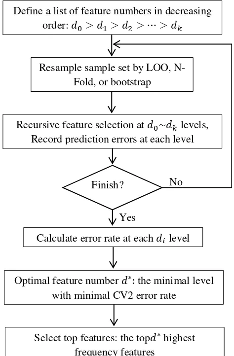
Zhang, et al., (2006) follow the CV2 scheme to estimate the error rate a teach level. In cross-validation experiments, different training subsets generate different lists of features (although many or most of them overlap in usual experiments). A frequency-based selection method is adopted to decide the lists of features to be reported. That is, after the recursive feature selection steps on each subset, we count at each of the
𝑑𝑖 levels the frequency of the features being selected among all rounds of cross-validation experiments. The top
𝑑𝑖 most frequently selected features are reported as the final 𝑑𝑖 features (called the top features).
In most situations, CV2 errors usually follow a U-shaped curve along the selection steps (feature numbers). Finding the minimal number of features that can give the minimal CV2 error rate is often desirable for
No
Yes
Define a list of feature numbers in decreasing order: 𝑑0>𝑑1>𝑑2 >⋯>𝑑𝑘
Resample sample set by LOO, N-Fold, or bootstrap
Recursive feature selection at 𝑑0~𝑑𝑘 levels, Record prediction errors at each level
Finish?
Calculate error rate at each 𝑑𝑖 level
Optimal feature number 𝑑∗: the minimal level with minimal CV2 error rate
Select top features: the top𝑑∗ highest frequency features
11 real applications. Another realistic consideration is the limited ability of follow-up biological investigations on the selected features. As a compromise, we decide the final number of features to be reported in an experiment by considering both the error rates and the limitation of follow-up biological investigations. The entire workflow is depicted in Figure 3.2; we call this whole scheme R-SVM (recursive SVM).
3.2
Random Forest
Random forests are a combination of tree predictors such that each tree depends on the values of a random vector sampled independently and with the same distribution for all trees in the forest. Random forest is an algorithm for classification developed by Breiman (2001) that uses an ensemble of classification trees. Each of the classification trees is built using a bootstrap sample of data, and each split the candidate set of variables is a random subset of the variables. Thus, random forest uses both bagging and random variable selection for tree building. The algorithm yields an ensemble that can achieve both low bias and low variance.
The random forests algorithm is: (1) draw ntree bootstrap samples from the original data, (2) for each of the bootstrap samples, grow an unpruned classification or regression tree, with the following modification: at each node, rather than choosing the best split among all predictors, randomly sample mtry of the predictors and choose the best split from among those variables (Bagging can be thought of as the special case of random forests obtained when mtry = p, the number of predictors), and (3) predict new data by aggregating the predictions of the ntree trees (i.e., majority votes for classification, average for regression).
12
3.2.1 Feature Selection Using Random Forest
Random forest returns several measures of variable importance, which were used by a few authors. Diaz-Uriarte & Andres (2006) found in (Dudoit & Fridlyand, 2003) and (Wu, et al., 2003) that they use filtering approaches and, thus, do not take advantage of the measures of variable importance returned by random forest as part of the algorithm. Diaz-Uriarte & Andres (2006) also found a similarity of variable importance measures in (Svetnik, Liaw, Tong, & Wang, 2004). However, their strategy is to achieve the accurate predictors, which might not be the most appropriate for a purpose as it shifts the emphasis away from selection the specific variables.
This feature selection strategy was proposed by Diaz-Uriarte & Andres (2006). The most reliable measure is based on the decrease of classification accuracy when values of a variable in a node of a tree are permuted randomly. To select features they iteratively fit random forests, at each iteration building a new forest after discarding those variables (features) with the smallest variable importance; the selected set of features is the one that yields the smallest out-of-bag (OOB) error rate.
It is proposed using out-of-bag estimates as an ingredient in estimates of generalization error. Assume a method for constructing a classifier from any training set. Given a specific training set T, from bootstrap training set𝑇𝑘, construct classifiers ℎ(𝒙,𝑇𝑘) and let these vote from the bagged predictor. For each 𝑦,𝒙in the training set, aggregate the votes only over those classifiers for which 𝑇𝑘 does not contain𝑦,𝒙. Call this the out-of-bag classifiers. Then the out-of-out-of-bag estimate for generalization error is the error rate of the out-of-bag classifier on the training set (Breiman, 2001).
Note that in this section they are using OOB error to choose the final set of features, not to obtain unbiased estimates of the error rate of this rule. Because of the iterative approach, the OOB error is biased down and cannot be used to assess the overall error rate of the approach, for reasons analogous to those leading to "selection bias" (Ambroise & McLachlan, 2002). The bootstrap strategy will be used to assess prediction error rates (see subsection 3.2.2).
3.2.2 Estimation of Error Rates in Feature Selection
13 carrying out variable selection. The .632+ bootstrap method was also used when evaluating the competing methods.
3.3
Partial Least Squares Discriminant Analysis (PLS-DA)
Partial Least Squares regression makes it possible to relate a set of dependent variables
𝑌=�𝑌1, … ,𝑌𝑝�to a set of independent variables 𝑋= {𝑋1, … ,𝑋𝑀} when the number of
independent and/or dependent variables is much larger than the number of observations. PLS regression consists in carrying out a principal components analysis of the set of variables 𝑋subject to the constraint that the (pseudo-) principle components of𝑋𝑗 are as "explanatory" as possible to the set of variables𝑌. It is then possible to predict 𝑌𝑘 from
𝑋𝑗by better separating the signal from the variable (Tenenhaus, Gauchi, & Ménardo, 1995). The goal of PLS regression is to provide a dimension reduction strategy in a situation where we want to relate a set of response variables 𝑌 to a set of predictor variables𝑋.
The PLS regression algorithm has been explained by some authors, such as Tenenhaus (1998) and Tenenhaus, Gauchi, & Ménardo (1995). The starting point is two data matrices 𝑋and𝑌. 𝑋is an 𝑁×𝑀matrix and 𝑌 is an 𝑁×𝑃matrix. Before the algorithm starts, the matrices should be scaled. The procedures are:
(1) Set 𝑋0= 𝑋 and 𝑌0 =𝑌
(2) Construct a linear combination of 𝑢1 from the 𝑌 columns and a linear combination of 𝑡1 from the 𝑋 columns that maximize𝑐𝑜𝑣(𝑢1,𝑡1) =𝑐𝑜𝑟(𝑢1,𝑡1).�𝑣𝑎𝑟(𝑢1). 𝑣𝑎𝑟(𝑡1). We obtain then two variables 𝑢1 and 𝑡1that correlate and resume well the variables
𝑋and 𝑌. We conduct then the regression:
𝑋0 =𝑡1𝑝′1+𝑋1
𝑌0= 𝑡1𝑟′1+𝑌1
(3) Re-process step 2 by replacing 𝑋0 and 𝑌0 with 𝑋1and 𝑌1. We will obtain new components: 𝑢2 as a linear combination from the 𝑌1 columns and 𝑡1 as a linear combination from the 𝑋1 columns. After conducting the regression, we will obtain the decomposition as follows.
𝑋0 =𝑡1𝑝′1+𝑡2𝑝′2+𝑋2
𝑌0 = 𝑡1𝑟′1+𝑡2𝑟′2+𝑌2
Iterate the procedure until the components obtained 𝑡1,𝑡2, … ,𝑡𝐴 explain sufficiently the variables𝑌. The components 𝑡ℎare the linear combinations of 𝑋 columns, which is also uncorrelated. The regression equation is:
14 Partial least squares discriminant analysis (PLS-DA) is a partial least squares regression of a set Y of binary variables describing the categories of a categorical variable on a set X of predictor variables (Pérez-Enciso & Tenenhaus, 2003). Although PLS was not originally designed for classification and discrimination purpose, some authors routinely use PLS for that purpose and there is substantial empirical evidence to suggest that it performs well in that role (Barker & Rayens, 2003). It is a compromise between the usual discriminant analysis and a discriminant analysis on the significant principal components of the predictor variables. This technique is specially suited to deal with a much larger number of predictors than observations and with multicolinearity, two of the main problems encountered when analyzing “omics” (such as transcriptomics, proteomics, and metabolomics) expression data.
3.3.1 Feature Selection based on Variable Importance in the Projection
When the number of independent variables is very large, it will give impact for PLS-DA analysis, even though we create components. That is because the impact of noisy data as well as redundancy data. Because of this reason, we still need to select several important variables before creating the components. Besides that, a fundamental requirement for PLS to yield meaningful answers is some preliminary variable selection. Enciso and Tenenhaus (2003) did this feature selection technique by selecting the variables on the basis of the Variable Importance in the Projection (VIP) for each variable.
By PLS regression model written as:
𝑌𝑘 =�(𝑋𝑤ℎ∗)𝑐ℎ
𝐻
ℎ=1
+𝑒
Where 𝑤ℎ∗is a p dimension vector containing the weights given to each original variable in the h-th component, and 𝑐ℎis the regression coefficient of 𝑌𝑘.
𝑉𝐼𝑃𝑗is a popular measure in the PLS literature and it is defined for variable j as:
𝑉𝐼𝑃𝑗 = �𝑝 � � 𝑅2(𝑦𝑘,𝑡ℎ)𝑤ℎ𝑗2 /� � 𝑅2(𝑦𝑘,𝑡ℎ)
𝑘 𝐻
ℎ=1 𝑘
𝐻
ℎ=1
� 1/2
15 In this study, we will analyze all three cases using PLS DA variables selection based on VIP. To select the number of variables selected, we use the criteria of R2, Q2, and accuracy rate. 𝑄ℎ2 is the value of Q2 for component h, and it can bedefined as:
𝑄ℎ2 = 1−𝑅𝐸𝑆𝑆𝑃𝑅𝐸𝑆𝑆ℎ
ℎ−1
Where 𝑃𝑅𝐸𝑆𝑆ℎ is the predicted sum of squares of a model containing h components, that also written as 𝑃𝑅𝐸𝑆𝑆ℎ= ∑𝑛𝑖=1(𝑦𝑖 − 𝑦�ℎ(−𝑖))2 and 𝑅𝐸𝑆𝑆ℎ−1 is the residual sum of
squares of a model containing h-1 components where𝑅𝐸𝑆𝑆ℎ =∑𝑛𝑖=1(𝑦𝑖− 𝑦�ℎ𝑖)2. 𝑄ℎ2is also used for selecting the number of components in the model, the number of PLS components will be selected if a new component satisfied 𝑄ℎ2 ≥0.05.
R2 (or cofficient of determination) is the fraction of the total variability explained by the model. R2 is defined as 𝑅2 = 1− 𝑅𝐸𝑆𝑆ℎ=1,..,𝐻⁄𝑆𝑆𝑇ℎ=1,…,𝐻, while 𝑆𝑆𝑇ℎ= ∑𝑛𝑖=1(𝑦𝑖 − 𝑦�ℎ𝑖)2. Beside that, Q2 is a measurement of the predictive ability of the model and it is obtained by:
𝑄2 = 1− � 𝑃𝑅𝐸𝑆𝑆ℎ
𝑅𝐸𝑆𝑆ℎ−1
𝐻
ℎ=1
𝑜𝑟 𝑄2 = 1− �(1−
𝐻
ℎ=1
𝑄ℎ2)
3.3.2 Sparse PLSDA (sPLS-DA)
The sparse PLS proposed by Lê Cao, Rossouw, Robert-Granié, & Besse (2008) was initially designed to identify subsets of correlated variables of two different types coming from two different data sets 𝑋 and 𝑌 of sizes (𝑛×𝑝) and (𝑛×𝑞) respectively. The original approach was based on Singular Value Decomposition (SVD) of the cross product𝑀ℎ =𝑋ℎ𝑇𝑌ℎ. Any real r-rank matrix 𝑀 (𝑝×𝑞) can decomposed into three matrices 𝑈,∆,𝑉as𝑀 =𝑈∆𝑉𝑇. One interesting property that will be used in sparse PLS method is that the columns vectors of 𝑈or 𝑢ℎand𝑉or 𝑣ℎ(called left and right singular vectors) correspond to the PLS loadings of 𝑋 and𝑌 if 𝑀 =𝑋𝑇𝑌.
Sparse loading vectors are then obtained by applying Lasso penalization on both 𝑢ℎ and
𝑣ℎ to perform variable selection. Indeed, one interesting property of PLS is the direct interpretability of the loading vectors as a measure of the relative importance of the variables in the model. The optimization problem of the sparse PLS minimizes the Frobenius norm between the current cross product matrix and the loading vectors:
min
𝑢ℎ,𝑣ℎ‖𝑀ℎ− 𝑢ℎ𝑣ℎ
′‖ 𝐹 2 +𝑃
𝜆1(𝑢ℎ) + 𝑃𝜆2(𝑣ℎ)
Where 𝑃𝜆1(𝑢ℎ) =𝑠𝑖𝑔𝑛(𝑢ℎ)(|𝑢ℎ|− 𝜆1)+ and 𝑃𝜆2(𝑣ℎ) =𝑠𝑖𝑔𝑛(𝑣ℎ)(|𝑣ℎ|− 𝜆2)+ are
applied componentwise in the vectors 𝑢ℎ and 𝑣ℎ and are the soft thresholding functions that approximate Lasso penalty functions. They are simultaneously applied on both loading vectors. The procedures of Sparse PLS are:
16 2. For h in 1 until H:
(a) Set 𝑀�ℎ−1 =𝑋ℎ−1𝑇 𝑌ℎ−1
(b) Decompose 𝑀�ℎ−1 and extract the first pair of singular vectors 𝑢𝑜𝑙𝑑 =𝑢ℎ and
𝑣𝑜𝑙𝑑 = 𝑣ℎ
(c) Until convergence of 𝑢𝑛𝑒𝑤 and 𝑣𝑛𝑒𝑤: i. 𝑢𝑛𝑒𝑤 =𝑃𝜆2(𝑀�ℎ−1𝑣𝑜𝑙𝑑), normalize 𝑢𝑛𝑒𝑤 ii. 𝑣𝑛𝑒𝑤 = 𝑃𝜆1(𝑀�ℎ−1𝑢𝑜𝑙𝑑), normalize 𝑣𝑛𝑒𝑤 iii. 𝑢𝑜𝑙𝑑 =𝑢𝑛𝑒𝑤, 𝑣𝑜𝑙𝑑 =𝑣𝑛𝑒𝑤
(d) 𝜉ℎ= 𝑋ℎ−1𝑢𝑛𝑒𝑤/𝑢𝑛𝑒𝑤′ 𝑢𝑛𝑒𝑤
𝜔ℎ= 𝑌ℎ−1𝑣𝑛𝑒𝑤/𝑣𝑛𝑒𝑤′ 𝑣𝑛𝑒𝑤
(e) 𝑐ℎ = 𝑋ℎ−1𝑇 𝜉ℎ/𝜉ℎ′𝜉ℎ
𝑑ℎ =𝑌ℎ−1𝑇 𝜉ℎ⁄𝜉ℎ′𝜔ℎ
𝑒ℎ =𝑌ℎ−1𝑇 𝜔ℎ/𝜔ℎ′𝜔ℎ
(f) 𝑋ℎ = 𝑋ℎ−1− 𝜉ℎ𝑐ℎ′
(g) Regression mode: 𝑌ℎ = 𝑌ℎ−1− 𝜉ℎ𝑑ℎ′ Canonical mode: 𝑌ℎ = 𝑌ℎ−1− 𝜔ℎ𝑒ℎ′
In the case where there is no sparsity constraint (𝜆1 =𝜆2 = 0) we obtain same results as in a classical PLS.
The extension of sparse PLS to a supervised classification framework is straightforward. It is possible to make an analysis of sparse PLS for discrimination purpose. The response matrix 𝑌 of size (𝑛×𝐾) is coded with dummy variables to indicate the class membership of each sample (Lê Cao, Boitard, and Besse, 2011).
Note that in this specific framework, we will only perform variable selection on the 𝑋 data set, i.e., we want to select the discriminative features that can help predicting the classes of the samples. The 𝑌 dummy matrix remains unchanged. Therefore, we set
𝑀ℎ =𝑋ℎ𝑇𝑌ℎand the optimization problem of the sPLS-DA can be written as: min
𝑢ℎ,𝑣ℎ‖𝑀ℎ− 𝑢ℎ𝑣ℎ
′‖ 𝐹 2 +𝑃
𝜆1(𝑢ℎ)
17
CHAPTER 4
METHOD OF ANALYSIS
In chapter 4, the method of analysis is described. Besides presentation of datasets used in this study, we also explain the statistical analysis including pre-processing data, R-programming, and interpretation.
4.1
Presentation of Datasets
Several datasets are needed to make sure the stability performance of our algorithms used, as mentioned that our objective is to compare the performance of four feature selection techniques in classification purpose. In term of this purpose, we use three datasets in this study containing human urines test, rat’s urines test, and rat’s plasma test. The first dataset contains 28 human urines which are analyzed by LC-MS (Metabolomic machine). There are two groups in this datasets, where group called “0” represents 14 human urines and group called “1“ represents the same 14 human urines in which 30 molecules are added. In this experiment, we measure 1271 features that we will then select some of which contributing the best in the classification.
The second dataset contains 20 rat’s urines which are also analyzed by LC-MS. Two groups named “contaminated” represents 10 rat’s urines occurring from rats contaminated in their drinking water by natural uranium and “not contaminated” represents 10 normal rat’s urines. In this experiment, 1376 features are measured and it will be selected several most important features. Last dataset contains the data obtained from 2x10 rat’s plasma with 810 features measured. It was collected from rats contaminated or not by natural natrium as described above. Overall, we use two type rats’ samples and one human sample and we use two type urines samples and one plasma sample.
4.2
Statistical Analysis
Statistical analysis steps include pre-processing data, R-programming, and interpretation. Step of pre-processing data explains the pre-action before analyzing using four features selection techniques for classification mentioned in chapter 3. R-programming step describes the R package used and the main idea of several functions created in software R. And last, step of interpretation explains two sides of interpretation view: statistical and biological interpretation.
4.2.1 Pre-Processing Data
18 useful for data treatment because each classification technique needs different requirement such as data centering, scaling, and transformation. As explained that R-SVM and RFFS don’t require any data transformation in analyzing procedure, it’s different with PLS technique, where both PLS-DA feature selection based on VIP and sPLS-DA, require pre-treatment data.
A recommended data transformation used for PLS-DA VIP and sPLS-DA is log10-pareto transformation, where we need two times data transformation. We transform the data to log10 and we use then Pareto scaling in log10 transformation data. Pareto scaling is defined as 𝑥�𝑖𝑗 = (𝑥𝑖𝑗 − 𝑥̅𝑖)⁄�𝑠𝑖 and it aims to reduce the relative importance of large values, but keep data structure partially intact (van den Berg, Hoefsloot, Westerhuis, Smilde, & van der Werf, 2006).
4.2.2 R-Programming
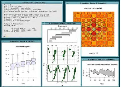
The process of statistical classification techniques is facilitated by software R. R is a language and environment for statistical computing and graphics. R provides a wide variety of statistical and graphical techniques, and is highly extensible. R is available as Free Software under the terms of the Free Software Foundation's GNU General Public License in source code form. It compiles and runs on a wide variety of UNIX platforms and similar systems (including FreeBSD and Linux), Windows and MacOS. R can be extended easily via packages. There are about eight packages supplied with the R distribution and many more are available through the CRAN family of Internet sites covering a very wide range of modern statistics (R-Foundation, 2014). Example of R screenshots is presented in Figure 4.1.
19 Before analyzing to main algorithms, we firstly create a decreasing ladder. The purpose of creating ladder is to define the variable selected based on decreasing function. In case 1 (human urines) for example, there are 26 iterations of features selected: 1271, 1017, 814, 651, 521, 417, 334, 267, 214, 171, 137, 110, 88, 70, 56, 45, 36, 29, 23, 18, 14, 11, 9, 7, 6, and 5 features. It is also carried out for rat’s urines dataset (26 iterations) and rat’s plasma dataset (24 iterations).
In this study, we use four core packages; it is one package for each technique. R-SVM: e107, RFFS: VarSel, PLS-DA feature selection based on VIP: DiscriMiner, and
sPLS-DA: mixOmics. Package e107 is functions for latent class analysis, short time Fourier
transform, fuzzy clustering, support vector machines, shortest path computation, bagged clustering, and also naive Bayes classifier (Meyer, et al., 2014). We use this package for developing the algorithm of Recursive SVM created by Zhang, et al., (2006). In analyzing of random forest for feature selection, package VarSel is proposed because this package is specially created by Diaz-Uriarte (2010) for this purpose. Unlike package e107 that we should develop the algorithm for analysis of R-SVM purpose, package VarSel is able to facilitate the users to analyze the datasets using RFFS directly without re-programming.
DiscriMiner is an R package created by Sanchez & Determan (2013) that has functions for discriminant analysis and classification purposes covering various methods such as descriptive, geometric, linear, quadratic, PLS, as well as qualitative discriminant analyses. We develop feature selection of PLS-DA based on VIP using this package. The main idea of this algorithm is the same as the idea of R-SVM algorithm. The different side is in the criteria of features ranking method. Package mixOmics is a package that provides statistical integrative techniques and variants to analyze highly dimensional data sets like sparse PLS-DA. This package is developed by (Dejean, Gonzalez, & Lê Cao, 2014). All R-code developed in this study is presented in Appendix 1.
4.2.3 Interpretation
20
CHAPTER 5
ANALYSIS RESULTS
Chapter 5 describes the results of analysis, which are divided into several sections. Section 1-4 explains the results obtained by each statistical technique. After that, section 5 shows the comparison performance of all techniques proposed. Finally, section 6 guides the readers in the biological interpretation and give the meanings of the study.
5.1
Analysis Using R-SVM
Recursive SVM (R-SVM) is an algorithm to recursively classifies the sample using SVM rules and selects the variables according to their weight in the SVM classifiers (Zhang, et al., 2006). The main objective of R-SVM is to select a subset of features with maximum discriminatory power between two classes. Since the feature dimension is large and the sample size is small, there are usually many combinations of features that can give zero error on the training data. Therefore, the “minimal error” cannot work. Intuitively, it is desirable to find a set of features that give the maximum separation between two classes of samples.
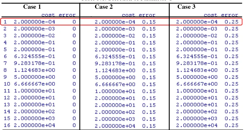
Table 5.1. Selection of Parameter C
Case 1 Case 2 Case 3
The SVM regularization parameter C is another challenge in SVM model selection. The parameter C determines the trade-off between minimizing the training error and reducing the model complexity. The range of C depends on the underlying SVM learning algorithm being used, but we see that the most appropriate C is the lowest. It is suggested that the most appropriate C range for SVM is between 10-2 and 104 (Huang, Lee, Lin, and Huang, 2007).
21 obtain the lowest error rate. In this C interval selected, there is no error rates change, it means that there is no different error rates obtained by using all point between 2.10-4 and 2.104 and we should select the lowest parameter C that is coloured red in Table 5.1, i.e., 2.10-4 for each case.
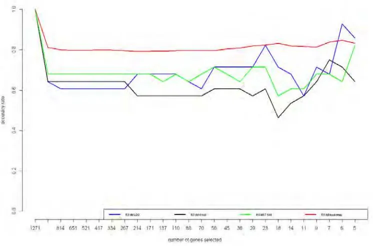
Figure 5.1. Human Urines Datasets Performance
Analyzing Human urines datasets (case 1), we will compare four cross-validation (CV) methods, i.e., leave-one-out (LOO), 4-fold, 7-fold, and bootstrap. Figure 5.1 represents the accuracy rates based on the number of features selected and CV methods used. The performance of 4-fold is the worst since it tends to obtain lowest accuracy rates. After that, 7-fold CV accuracy rates obtained is also quite poor even though it is better than 4-fold CV performance. The most stable and quite good is the performance of bootstrap since it leads to 80 percent and there is no much fluctuation. However, since it fluctuates, the performance of LOO is able to reach around 90 percent that has never been achieved by other CV methods.
We can see the accuracy rates for each CV used and features selected in Table 5.2. Using all features leads to obtain maximum accuracy rates, the result that quite contradict to our hypotheses. To better known, we will show the conclussion after describing all results. In this step, we see there is a significant decreasing performance using between all features (1271 features) and the second level (1017 features).
22
Table 5.2. Human Urines Accuracy Performance
In human urines dataset (Table 5.2), we can choose six features (LOO), seven features (4-Fold), five features (7-Fold), and six features (bootstrap) for low-level, while selecting 56 features (LOO, 4-Fold, and 7-Fold) and 88 features (bootstrap) for middle-level. In this case, we know that the performance of low-level is higher than the performance of middle-level, even for high-level. By using 6 features, the accuracy performance obtained by LOO CV could achieve 93 percent, that means there are 26 samples classified correctly, and there are just two samples classified incorrectly.
23 In case 2, Rat’s urines dataset, the performance of accuracy using RSVM is poorer than Human urines dataset although it is more stable. The performance of 4-Fold and 5-fold seems similar, while it looks also similar for the performance of bootstrap and LOO. The best accuracy rates is achieved by LOO in around 85 percent (See Figure 5.2).
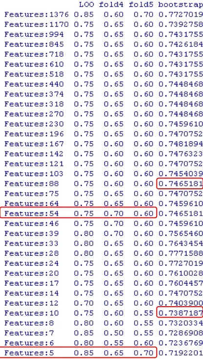
Table 5.3. Rat’s Urines Accuracy Performance
There is like a confusing in classification while using thousand features, when the features are highly corelated and redundant. It can be shown that the result using many features do not always tend to achive a better accuracy than using few features. If we could select the most appropriate features, although it is not many, we could achive a good or even better than using high-level features.
24
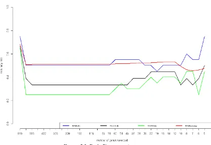
Figure 5.3. Rat’s Plasma performance
Recursive SVM as a selection variable technique based on SVM rules could not achieve a quite good in our last dataset, i.e, Rat’s plasma dataset (case 3). The accuracy performance is always under 80 percent. Besides that, by observing all three cases, we can see that the performance of N-fold is always poorer than bootstrap and LOO. The performance of bootstrap and LOO is quite similar, but LOO always leads to the best accuracy (See Figure 5.3).
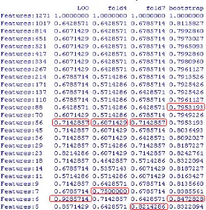
In Rat’s plasma dataset (Table 5.4), it is shown that RSVM couldn’t achieve a good results since the accuracy is around 50 percent. The highest accuracy is obtained by LOO CV that achieve just 75 percent, that means 15 samples are classified correctly, and 5 samples are not. For low-level, we can choose five features (LOO, 4-fold, and fold), and twelve features (bootstrap), while selecting 51 features (LOO, 4-Fold, and 5-Fold) and 60 features (bootstrap) for middle-level.
25
Table 5.4. Rat’s Plasma Accuracy Performance
To compare all CV method, it is shown two types point of view, which are in accuracy rates comparison point of view (Table 5.5) and features selected point of view (Figure 5.4). We would like to describe the low-level analysis, while middle-level analysis is presented in Appendix 2d.
Human urines datasets is able to be classified well by using RSVM since it is confirmed that the two classes are able to be differentiated easily. That is why the accuracy rates obtained is highest. In other side, Rat’s plasma dataset achieves poorest accuracy since the two clases are more complicated. Comparing to the other CV methods, LOO always leads the best performance, quite different with other CV methods achieved.
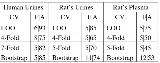
Table 5.5. Summary of RSVM low-level Result Human Urines Rat’s Urines Rat’s Plasma
CV F|A CV F|A CV F|A LOO 6|93 LOO 5|85 LOO 5|75 4-Fold 8|75 4-Fold 5|65 4-Fold 5|50 7-Fold 5|82 5-Fold 5|70 5-Fold 5|45 Bootstrap 5|85 Bootstrap 11|74 Bootstrap 12|53
26
Figure 5.4. Comparison of features selected in : (a) Human Urines datasets, (b) Rat’s Urines datasets, and (c) Rat’s Plasma datasets
To better understand about the meaning, we make a venn diagram of features selected that is devided by CV methods used for each case (See Figure 5.4). The features selected are quite similar for 4 CV methods used in each case (detailed in Table 5.6). Figure 5.4a shows that LOO selects four features that are also selected by other three cv methods (even there are 5 features same with 4-fold and 7 fold, and also 5 features which are same with bootstrap). In addition, LOO selects the features which are exactly selected by other three cv methods. It means that LOO is really the most appropriate CV methods in low-level analysis because they use similar features to classify the dataset and LOO is able to achieve much higher.
Table 5.6. The Common Features Selected by RSVM Human Urines M302T478 M310T428 M207T97 M169T41
Rat's Urines M180T194 M194T256 M338T217 M340T269 M206T158 Rat's Plasma M875T275_1 M494T437 M496T473 M524T539 M524T551
5.2
Analysis Using Random Forest for Feature Selection (RFFS)
Random forest is an algorithm for classification developed by Leo Breiman that uses an ensemble of classification trees. Each of the classification trees is built using a bootstrap sample of data, and each split the candidate set of variables is a random subset of the variables. Thus, random forest uses both bagging and random variable selection for tree building. The algorithm yields an ensemble that can achieve both low bias and low variance.
Random forest returns several measures of variable importance. The most reliable measure is based on the decrease of classification accuracy when values of the variable
(a) (b)
27 in a node of tree are permuted randomly. To select features, we iteratively fit random forest, at each iteration building a new forest after discarding those variables with the smallest variable importance. The selected set of features is the one that yields the smallest Out-of-Bag (OOB) error rate.
Table 5.7. Analysis using Feature Selection Random Forest
As shown in Table 5.7, when using high-level features, the OOB error rates obtained are quite poor. It indicates that using high-level features (even all features) is not proposed. OOB error rates decrease almost linearly with the decreasing of features level selected. After all, we choose five features for each case (human urines, rat’s urines, and rat’s plasma) because it leads to get minimum error rates. Besides that, we should see that the performance of middle-level is not better than low-level performance.
Since it is confirmed that two classes of Human Urines datasets could be differentiated easily, the error rates obtained is always zero, even for low level. It means that, by just using five features, all 28 samples are classified correctly. Although RFFS could not achieve zero error rates, the performance is still satisfied since it achieves 0.05 error rates for Rat’s Urines datasets and Rat’s Plasma datasets. Analyzing these two datasets, it means RFSS is able to classify the 19 samples correctly, and just one sample is not.
28
5.3
PLS-DA Feature Selection based on VIP
Partial Least Squares regression makes it possible to relate a set of dependent variables to a set of independent variables when the number of independent and/or dependent variables is much larger than the number of observations. However, when the number of independent variables is very large compare to the number of observation, it will give impact for PLS-DA analysis, even though we create components. That is because the impact of noisy data as well as redundancy data. Because of this reason, PLS-DA is not sufficient and we still need to select several important variables before creating the components. Besides that, a fundamental requirement for PLS to yield meaningful answers is some preliminary variable selection. Enciso and Tenenhaus (2003) did this feature selection technique by selecting the variables on the basis of VIP for each variable.
After using machine learning analysis, in this part, we would like to show the result analysis of our three datasets treatment using supervised classification, i.e., PLS-DA feature selection technique based on VIP and sPLS-DA for next section.
Not like machine learning rules that use only accuracy rates as performance criteria, we use also two other criteria, i.e., R2, Q2, since the estimation of accuracy is overestimed in PLS-DA. It is also shown in Figure 5.5 that this method could reach 100 percent for almost all feature levels selected for all three cases. After all, to select the number of features, we select the levels that produce the largest R2, Q2, and accuracy rate, with the closest distance between R2 and Q2.
29 To obtain the optimum result, we choose different number of components selected for each level using Q2j criterion (the PLSDA model having the highest Q² was kept). This idea is logic where each level of selected features defines different number of selected components.
Analyzing human urines dataset, the accuracy rate obtained is very perfect when using all features (see Table 5.8). However, we can see in Figure 5.5 that there is a relatively large distance between R2 and Q2 in this level which indicates selecting all features is not the best choice, as also shown in RFSS analysis. We surmise that there is a significant effect of noisy data in this level. This phenomena is also happened in rat’s urines and rat’s plasma dataset (see Figure 5.5), where the largest distance is placed in the first level when using all features.
The distance go downly by the decreasing number of variables selected. As stated that Human urines dataset is clearly differentiated both in two classes, so the performance is always well in almost all levels. Analyzing rat’s urines and rat’s plasma datasets, we can see that about 200 features selected, the distance fluctuates smoothly in low value. We indicates that the best choice is to select the features around five and 200 features.
Table 5.8. Human Urines Dataset’s Selected Components and It’s Performance
30 classes variability is explained by the model with predictive ability that’s equal to 99.4 percent. It does not have a big difference with middle level using three components from 56 features selected (the model can explain 99.9 percent of total variability and has 99.5 percent of predictive ability).
Table 5.9. Rat’s Urines Dataset’s Selected Components and It’s Performance
Like Human urines dataset, the number of components selected of rat’s urines dataset (Table 5.9) has a particular pattern like Bell-shape, where it starts selecting with small number of components for high level, increase in middle level, and decrease in low level. It is also happening for our rat’s plasma dataset (shown in Table 5.10).
31
Table 5.10. Rat’s Palsma Dataset’s Selected Components and It’s Performance
PLS-DA feature selection based on VIP is a technique that could achieve well the accuracy rate, as well as the score of R2 and Q2. In low level, This model can explain 89 percent total variability of rat’s urines classes and 83 percent of rat’s plasma classes, while it has a predictive ability of 84 percent for rat’s urines dataset and 80 percent for rat’s plasma dataset. List of features selected is presented in Appendix 3.
5.4
Sparse PLS-DA (sPLS-DA)
sPLS-DA is based on Partial Least Squares (PLS) Regression for discrimation analysis, but a lasso penalization has been added to select variables. Lê Cao, Boitard, and Besse (2011) showed that sPLS-DA is extremely competitive to the wrapper methods. In addition, the computational efficiency of sPLS-DA as well as the valuable graphical outputs that provide easier interpretation of the results make sPLS-DA a great alternative to other types of variables selection techniques in a supervised classification framework. In this part, we would like to show the the result of sPLS-DA analysis in our three datasets.
32
Figure 5.6. The Performance Using sPLS-DA Analysis
Since sPLS-DA works with loading factors to select the features, it optimizes the selection of features by computing the PLS-DA model. This method affects to the better selection of PLS-DA model for each level, indicated by similar value obtained of R2 and Q2 in Figure 5.6.
Table 5.11 shows the performance of human urines classification. sPLS-DA is able to choose the features based on the loading factors from each iteration. This technique is quitely surprising since it produce very good performance, in either variability explanation performance, predictive ability, or accuracy rate. Unlike PLS-DA feature selection based on VIP, the number of components selected in sPLS-DA does not follow Bell-shape. Because the performance is very well for all levels (the criteria is always more than 98 percent), it doesn’t matter to choose the lowest level of feature selection. Basicly, the different class is differentiated clearly so that a low level of features selected is sufficient.
33
Table 5.11. Human Urines Dataset’s Selected Components and It’s Performance
In low-level, we can be satisfied by selecting ten features (5 components), while we consider to choose 60 features (4 components) in middle-level. By using ten features, the model can explain 90 percent of the total variability of rat’s urines different classes with 91 percent of predictive ability. Therefore, sPLS-DA model is able to explain 94 percent of the total variability of rat’s urines different classes with 94 percent of predictive ability in middle-level (see Table 5.12).
34 Rat’s plasma dataset is also analyzed using sPLS-DA technique in features selection purpose. The result is presented in Table 5.13. Like rat’s urines, this classification is diffetentiated by two classes, contaminated and not contaminated plasma. By all four criteria, we choose nine features in low level (five components) and 70 features (three components) in middle level that is presented in Appendix 3.
In low level, the model can explain 99 percent of the total variability of rat’s plasma different classes with 99 percent of predictive ability. Therefore, sPLS-DA model is able to explain 94 percent of the total variability of rat’s plasma different classes with 94 percent of predictive ability in middle-level.
sPLS-DA working way by selecting the features and creating the components from loading factors achieves very well the accuracy rate, as well as the score of R2 and Q2. In low level, This model can explain at least 90 percent total variability and it has a predictive ability more than 94 percent. In addition, this model could achive a hundred percent of accuracy rate for all three cases.
Table 5.13. Rat’s Plasma Dataset’s Selected Components and It’s Performance
5.5
Methods Comparison
35 Both in machine learning and supervised classification techniques used in this study, one solution proposed is to reduce the dimensionality of the data either by performing features selection, or by introducing artificial variables (i.e. latent variables). The purpose of the features or variables selection is to eliminate irrelevant variables to enhance the generalization performance of a given algorithm (Rakotomamonjy, 2003) as well as to gain some insight about the concept learned (Diaz-Uriarte & Andres, 2006). Other advantages of feature selection and introducing artificial variables include cost reduction of data gathering and storage, and also on computational speedup. We choose the machine learning technique, i.e., RSVM and RFFS, as proposed techniques in features selection and supervised classification technique, i.e., PLS-DA VIP and sPLS-DA, as the technique of introducing artificial variables.
After one-by-one technique interpretation section, we would like to compare all performance techniques used in classifying our three datasets. We consider three point of views to evaluate our three techniques : (1) Accuracy rates (R2 and Q2 for supervised classification techniques), (2) Computational time needed, and (3) Similarity of features selected. After all, one main point, we would like to evaluate our four techniques by biological interpretation for the next section to gain some insight and meaning about the concept learned.
Table 5.14. Low-level Performance Comparison
Method Human Urines Rat’s Urines Rat’s Plasma RSVM-LOO 6 (92,86%) 5 (85,00%) 5 (75,00%) RSVM-Bootstrap 6 (84,73%) 10 (73,87%) 12 (53,21%) RSVM-4Fold 7 (75,00%) 5 (65,00%) 5 (50,00%) RSVM-7(5)Fold 5 (82,14%) 5 (70,00%) 5 (45,00%) RFFS 5 (100%) 5 (95,00%) 5 (95,00%) PLS-DA VIP 5 (99,60%|99,44%) 8 (89,12%|84,44%) 6 (82,70%|79,59%) sPLS-DA 5 (99,69%|99,69%) 10 (89,52%|90,64%) 9 (99,15%|99,05%) Notes : number of features selected (accuracy) – for machine learning; number of features
selected (R2 | Q2) – for supervised classfication
In machine learning techniques proposed, the performance of RFFS is always leading since it reachs more than 95 percent correctly classified samples, either in low-level analysis (Table 5.14) or middle-level analysis (Table 5.15). The performance of RSVM is quite good for LOO, but it is poor for other three CV methods used, particularly these three methods performance is very poor for middle-level analysis. Analyzing supervised classification techniques, PLS-DA VIP and sPLS-DA could achieve a good performance since both of them could reach more than 90 percent for R2 and 80 percent Q2 in low-level (Table 5.14). In addition, these techniques could reach more than 94 percent for R2 and 89 percent Q2 in middle-level (Table 5.15). sPLS-DA performance is quite better than PLS-DA VIP in low-level, but they are both similar in middle-level.
36 features). Despite RSVM N-Fold could achieve small set (five features), it is not an appropriate method in this study because of their poor performance. The number of features selected in supervised classification techniques (low-level analysis, see Table 5.13) is similar, although PLS-DA could achieve little smaller set of features.
Table 5.15. Middle-level Performance Comparison
Method Human Urines Rat’s Urines Rat’s Plasma RSVM-LOO 56 (71,43%) 54 (75,00%) 51 (55,00%) RSVM-Bootstrap 88 (79,53%) 88 (76,45%) 60 (51,52%) RSVM-4Fold 56 (60,71%) 54 (70,00%) 51 (33,33%) RSVM-7(5)Fold 56 (71,43%) 54 (60,00%) 51 (35,00%) RFFS 56 (100%) 94 (95,00%) 56 (90,00%) PLS-DA VIP 56 (99,92%|99,49%) 60 (99,49%|94,06%) 87 (99,24%|88,59%) sPLS-DA 56 (99,01%|99,01%) 60 (94,34%|94,32%) 70 (94,16%|93,72%) Notes : number of features selected (accuracy) – for machine learning; number of features
selected (R2 | Q2) – for supervised classfication
The number of features selected by machine learning techniques, we can say, is smaller than the number of features selected by supervised classification techniques, except for RSVM-bootstrap. In the middle-level analysis (Table 5.15), N-fold and LOO RSVM achieve the smallest set, while bootstrap RSVM achieves the biggest set of features selected. The number of features selected by RFFS is a little bigger than N-Fold and LOO RSVM, but it is still in the normal range. As low-level analysis, the number of features selected in supervised classification techniques is similar. However, sPLS-DA could achieve now little smaller set of features, as an opposite of low-level analysis.
Table 5.16. Computational Time Comparison (Minutes)
Method Human Urines Rat’s Urines Rat’s Plasma
RSVM-LOO 8 4 12
RSVM-Bootstrap 29 10 32
RSVM-4Fold 1 1 1
RSVM-7Fold (5Fold) 1 1 1
RFFS 1 1 1
PLS-DA VIP 8 12 15
sPLS-DA 4 3 6
37
Figure 5.7. The number of features selected for low-level analysis based on technique used for : (a) Human urines dataset, (b) Rat’s urines dataset, and (c) Rat’s plasma dataset
Having compared the accuracy (R2 | Q2), number of features selected, as well as computational time, it is also important to know the similarity of features selected based on each teachnique proposed. In section 5.1, we did the comparison of features selected based on CV methods used in RSVM and it shows the strong similarity of features selected. Because of this reason, we use only RSVM-LOO in this section since it performs best for RSVM method for low-level analysis.
Analyzing Figure 5.7a, the features selected by each technique is strongly independent since they choose different features based on their own way. This result is followed by other cases (see Figure 5.7b and Figure 5.7c) although it is not as strongly different as human urines features selection performance. Since low-level analysis presents fewer than 15 features for each technique, it is important to know their similarity in middle-level.
Table 5.17. The Similarity of Features Selected in Middle-level Analysis (%) Method Human Urines Rat’s Urines Rat’s Plasma
RSVM 18 18 14
RFFS 50 51 70
PLS-DA VIP 77 82 51
sPLS-DA 57 35 26
(a) (b)