Approximations of the Carrier–Greenspan periodic solution to the shallow water wave equations for flows on a sloping beach.

Published online 9 June 2011 in Wiley Online Library (wileyonlinelibrary.com/journal/nmf). DOI: 10.1002/fld.2607

Approximations of the Carrier–Greenspan periodic solution to the

shallow water wave equations for flows on a sloping beach

Sudi Mungkasi

1,2,*,†

and Stephen G. Roberts

1

1_{Mathematical Sciences Institute, The Australian National University, Canberra, Australia} 2_{Department of Mathematics, Sanata Dharma University, Yogyakarta, Indonesia}

SUMMARY

The Carrier–Greenspan solutions to the shallow water wave equations for flows on a sloping beach are of two types, periodic and transient. This paper focuses only on periodic-type waves. We review an exact solution over the whole domain presented by Johns [‘Numerical integration of the shallow water equations over a sloping shelf’,Int. J. Numer. Meth. Fluids, 2(3): 253–261, 1982] and its approximate solution (the Johns pre-scription) prescribed at the zero point of the spatial domain. A new simple formula for the shoreline velocity is presented. We also present new higher order approximations of the Carrier–Greenspan solution at the zero point of the spatial domain. Furthermore, we compare numerical solutions obtained using a finite volume method to simulate the periodic waves generated by the Johns prescription with those found using the same method to simulate the periodic waves generated by the Carrier–Greenspan exact prescription and with those found using the same method to simulate the periodic waves generated by the new approximations. We find that the Johns prescription may lead to a large error. In contrast, the new approximations presented in this paper produce a significantly smaller error. Copyright © 2011 John Wiley & Sons, Ltd.

Received 14 May 2010; Revised 14 April 2011; Accepted 15 April 2011

KEY WORDS: sloping beach; periodic waves; shallow water wave equations; finite volume methods; fixed boundary; moving shoreline

1. INTRODUCTION

The Carrier–Greenspan periodic solution [1] has been widely applied to test the performance of numerical methods used to solve the shallow water wave equations (consult [2–6] for example). This solution involves a fixed boundary and a moving boundary. To generate the periodic waves, either the Carrier–Greenspan exact solution or its approximation at the fixed boundary is prescribed. Johns [5] presented a specific form of the Carrier–Greenspan exact solution of periodic type over a spatial domain and prescribed an approximate solution at the zero point of the spatial domain, where the fixed boundary is located. The approximate solution can be applied at the fixed boundary to generate an approximation of the Carrier–Greenspan exact solution using a numerical method as done by a number of authors, such as Johns [5] and Sidén and Lynch [6]. Thus, the numerical solution is affected by two sources of error, namely, the error in the boundary condition (at the fixed boundary) and the error introduced by the numerical discretization. Ideally, when testing a numer-ical method, we want to quantify the error introduced by the numernumer-ical discretization. However, testing a numerical method by prescribing the approximate solution at the fixed boundary may be misleading because the error in the boundary condition could be the dominant term. Note that the prescription at the fixed boundary propagates towards the moving boundary (shoreline), so the error at the fixed boundary also propagates towards the shoreline.

*Correspondence to: Sudi Mungkasi, Mathematical Sciences Institute, The Australian National University, Canberra, Australia.

Our main point is that, in general, the approximate solution of Johns [5] is unable to accurately estimate the Carrier–Greenspan exact solution at the zero point of the spatial domain. In addition, the large prescription error at the fixed boundary results in a large error of the solution generated by the numerical method. Therefore, we propose new approximations (which are more accurate than the approximate solution of Johns [5]) of the Carrier–Greenspan exact solution at the zero point of the spatial domain.

In this paper, we derive the formulation of Johns [5] for the Carrier–Greenspan periodic solution, as Johns [5] did not explicitly present the derivation. Based on that formulation, we then derive a new formula for the shoreline velocity and new approximate solutions at the zero point of the spatial domain. The new formula for the shoreline velocity is found using l’Hospital’s Rule, and the new approximate solutions at the zero point of the spatial domain are found by extending the approximate solution of Johns [5] using either formal expansion or fixed point iteration.

The remainder of this paper is organized as follows. Section 2 recalls the shallow water wave equations in dimensional and dimensionless systems. Section 3 is devoted to the analytical work on the Carrier–Greenspan solution for periodic waves. In Section 4, two test cases are investigated, which verify our claim that the use of the Johns prescription can lead to large errors, and in addition, our new approximations are indeed more accurate. In Section 5, we present the rate of convergence of the numerical method used in the simulations. Finally, some concluding remarks are stated in Section 6.

2. GOVERNING EQUATIONS

The shallow water wave equations can be written in the standard dimensional system as well as the non-standard dimensionless system. These equations are the mathematical relations governing the vertically averaged hydrostatic water motion. In this section, we recall the shallow water wave equa-tions in both systems. Equaequa-tions in the dimensionless system are used for simplicity in the analytical work in Section 3, whereas equations in the dimensional system are utilized to easily understand the solution, physically, in the numerical experiments in Sections 4 and 5.

In the standard Cartesian coordinate system, the conservative shallow water wave equations consist of the mass and momentum equations

h_tC

hu

xD0, (1)

hu_tC

hu2_C1 2gh

2

x

D gh´_x. (2)

Here,x_{represents the coordinate in one-dimensional space, trepresents the time variable,uD}

u_{.x,t/denotes the water velocity,´D´.x/denotes the water bed topography,hDh.x,t/} denotes the water height, that is, the distance from the free surface to the water bed topography, and

gis the constant of gravitation.

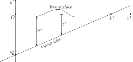
Consider the situation illustrated in Figure 1. The topography changes linearly withx

´_D.h

0=L/xh0, (3)

in whichh

0 is the vertical distance from the originO to the topography at any time, andLis the

horizontal distance from the originO to the topography when the water is still. This implies that when the water is still,´_{Dhover the spatial domain,´Dh}

0 atxD0, and the position of the

shoreline isx_DL.

We introduce a new variable called the stagew_{WDhC´, which specifies the free surface.} Scaling the horizontal distance by L_{, the vertical distance by h}

0, the time by L= p

gh 0, and

the velocity bypgh

0, we can rewrite Equations (1) and (2) as the nonconservative dimensionless

shallow water wave equations

Figure 1. Cross section of a sloping beach.

utCuuxCwxD0. (5)

In this paper, all unstarred variables denote dimensionless quantities corresponding to their dimen-sional quantities denoted by starred variables. Equations (4) and (5) were used by Johns [5] in developing a finite difference numerical technique to simulate shallow water flows on a sloping beach.

Remark 1

For smooth solutions, Equations (4) and (5) are equivalent to the conservative dimensionless shallow water wave equations

htC.hu/xD0, (6)

.hu/_tC

hu2_C1 2h

2

x

D h´x. (7)

3. PERIODIC WAVES ON A SLOPING BEACH

In this section, we review the solutions for periodic waves on a sloping beach presented by Carrier and Greenspan [1]. Five subsections are given. In Subsection 3.1, we recall the hodograph trans-formation applied by Carrier and Greenspan [1] to solve the shallow water equations analytically. This solution in the hodograph variables is then transformed back to the physical variables in Sub-section 3.2 to get the formulation of Johns [5] for the Carrier–Greenspan periodic solution. We then present a new formula for the shoreline velocity in Subsection 3.3. In Subsection 3.4, we review the Johns approximation, which can be used as boundary conditions for numerical simulations, to the Carrier–Greenspan periodic solution atx_D0. Finally, Subsection 3.5 is devoted to new (more accurate) approximations of the Carrier–Greenspan periodic solution atx_D0.

3.1. Carrier–Greenspan solution

Carrier and Greenspan [1] applied the classical hodograph transformation to solve the shallow water wave equations. Two dimensionless hodograph variables

_D4c, (8)

_D2.u_Ct / (9)

were used. Here,

c_Dpw_C1x (10)

is the wave speed relative to the water velocityu. In the hodograph system, the variables and

actually the water heighthin our dimensionless system. The dimensionless variables are related to the hodograph variables as

x_D1 4

1 16

2 1

2u 2

C1, t_D1

2u, (11)

w_D1 4

1 2u

2

, u_D1, (12)

where_D .,/is a potential function satisfying

. / D0. (13)

Equations for stage w and velocity u given by Equation (12) are the Carrier–Greenspan exact solution. The choice of .,/, which satisfies Equation (13), depends on the conditions of the investigated problem.

Carrier and Greenspan [1] showed that a periodic oscillation of water is formed if we take

.,/_DAJ0.! /cos.!/ (14)

as long as the Jacobian@ .x,t / =@ .,/does not vanish in >0. This means that the implicit func-tionsw.x,t /andu.x,t /are single-valued, that is, the waves represented by those functions do not break. Here,J0is the Bessel function of the first kind of order0. The constant!is given by=T

instead of the usual value2=T because a coefficient of 2 has appeared in the definition ofin Equation (9), whereT is the dimensionless period of oscillation. According to Equations (13) and (14), we can infer that

.,/_DAJ0.! /sin.!/ (15)

is also a potential function satisfying Equation (13).

3.2. The formulation of Johns for the Carrier–Greenspan periodic solution

In this subsection, we transform the solution (12) from the hodograph variablesandto the usual variablesxandt.

Considering the potential function (15), Johns [5] presented the corresponding Carrier–Greenspan periodic solution and prescribed an approximation of the Carrier–Greenspan periodic solution at

x_D0. Here, we derive the formulation‡ _{of Johns [5] for the Carrier–Greenspan periodic solution,}

so that in the next subsections we can propose a new formula for the shoreline velocity, review the prescription of Johns atx_D0, and propose new approximations of the Carrier–Greenspan periodic solution atx_D0. The motivation here is to provide the missing derivation of the solution presented by Johns [5].

Let us consider the potential function (15). Its partial derivatives are

D !AJ1.! /sin.!/, (16)

D!AJ0.! /cos.!/, (17)

whereJ1 andJ0are Bessel functions of the first kind of order 1 and 0, respectively. Substituting

Equations (16) and (17) into Equation (12), we obtain

w_D 1 2u

2 C1

4!AJ0.! /cos.!/, (18)

u_D !AJ1.! / ent from that used by Carrier and Greenspan [1]. Equations (20) and (21) are the Carrier–Greenspan exact solution corresponding to the potential function (15).

For convenience, we rewrite the Carrier–Greenspan exact solutions (20) and (21) as

w_D 1

3.3. Calculating the stage and velocity

Let us recall some properties of the shoreline before presenting how to calculate the stagew and velocityuover the whole domain. The shoreline is a moving boundary, and its position is defined at any time byc_D0, so that, introducing the dimensionless horizontal displacementof the shoreline, by Equation (10), we have

.t /_Dw.1_C .t /,t /. (24)

Differentiating Equation (24) with respect tot, we have

d

dt Dwx

d

dt Cwt. (25)

Using Equation (4) and assuming thatwx.1C .t /,t /<1, we obtain the kinematical condition of the

shoreline

u_Dd

dt at xD1C. (26)

A statement of zero depthc_D0atx_D1_C and the kinematical condition (26) are the boundary conditions at the shoreline [5]. Note that because the slope of the topography in the dimensionless system is unity, we have_Dw at the shoreline, as described by Dietrich, Kolar, and Luettich [4]. This means that the horizontal displacement of the shoreline is equal to the vertical displacement of the shoreline. Because the instantaneous shoreline is fixed by the statement of zero depthc_D0at

x_D1_C, the horizontal displacement of the shoreline is

To test a numerical method, Dietrichet al.[4] used the Carrier–Greenspan solution by referring to the formulation§_{of Johns [5]. To figure out the solution, Dietrichet al.[4] took two steps. First, the}

system of equations consisting of the horizontal displacementand the velocityuof the shoreline

_D 1

were solved. Equation (29) was solved for velocityuusing a finite difference approximation on the du=dt terms as well as using the information that the velocity of the shoreline at maximum inun-dation is zero. The shoreline displacement was found by substituting the shoreline velocityuinto Equation (28). Second, the stagewand velocityuat the interior points in the wet region (on the left side of the shoreline) were calculated using Equations (22) and (23).

Here, we propose a different approach at the first step to find the shoreline velocity. Let us con-sider the velocity formulation (21) at wet areas, that is, on the interval˛>0. We take the limit of the velocity formulation (21) as˛goes to zero and take l’Hospital’s Rule to get

u_D 2

which is our new formula for the shoreline velocity. Note that we take Equation (21), instead of Equation (23), into consideration in the derivation of Equation (30) because it is clearer to work with. Then the shoreline displacement is found by substituting the shoreline velocityuinto Equa-tion (28). The second step is similar to the work of Dietrichet al.[4]. To be specific, we can use the Newton–Raphson method to solve Equations (22) and (23) to get the stagewand velocityuof interior points in the wet region, with a note that the solution at a point closer to the shoreline is the initial guess for the Newton–Raphson method in obtaining the solution for a point further away from the shoreline.

3.4. The Johns approximate solution at the zero point of the spatial domain

In this subsection, we focus on the solution at spatial pointx_D0and review the prescription of Johns [5] defined at that point.

Let us assume thatw,u<<1atx_D0. Atx_D0, Johns [5] prescribed the stage

whereis the dimensionless wave amplitude, and fixed the amplitude factorAin terms of, which can be explained as follows. Let

w_Dw0Cıw , uDu0Cıu (32)

be defined, wherew_Dw0,uDu0 is a reference state, whereasıwandıuare perturbation terms.

Substituting Equation (32) into the right-hand side of Equations (22) and (23) with a sea at rest

w0D0,u0D0as the reference state leads to

u_D

which are explicit functions of timet and linear with respect to the amplitudeA_{. This means that} all contributions of perturbation termsıwandıuon the right-hand side of Equations (33) and (34) are neglected.

Matching Equation (35) with Equation (31), Johns [5] fixed

A_D

J04_T

, (37)

which is the amplitude factorAin terms of. We note that the assumption made onwanduin the linearization of Johns (w,u << 1atx_D0) impliesA<< 1. However, the amplitude factorAgiven by Equation (37), which implies the quality of approximation (35) and (36), is determined by two elements. The first is, rather intuitively, the magnitude of, whereas the second is the denominator

J0.4=T /. As a result, we can have significant nonlinear effects even for moderate values of ,

which will be demonstrated in Section 4.

In this paper, Equation (35) is called ‘the Johns approximate solution’ of the Carrier–Greenspan exact solution for the stagew at x_D0 or ‘the Johns prescription’ when it is applied at a fixed boundary to generate a periodic wave using a numerical method. Note that the value of the ampli-tude factorA_{corresponds to the maximum shoreline displacement (see the explanation of Carrier} and Greenspan [1] for more details). That is, the shoreline horizontal position varies from1_jA_jto

1_CjA_j.

3.5. More accurate approximations at the zero point of the spatial domain

In this subsection, we extend the Johns approximate solution, which is defined atx_D0, to get more accurate approximations. We describe two ways to do this extension. The first is by formal expan-sion of stagew and velocityuwith respect to the amplitudeA, and the second is by a fixed point iteration with a sea at rest (w0D0,u0D0) as the initial guess of the solution. (Please note that one

may also use other standard methods, such as the Newton–Raphson method, for solving a system of equations to do an extension of the Johns approximate solution.)

The extension by formal expansion follows. Suppose that we are interested in getting an approx-imation that is quadratic with respect to the amplitudeA_{. The motivation is that we want to add an} extra term to the approximate prescription (35) of Johns [5], so that it results in a new approximation that is a second order of accuracy. Let

w_Dw.A/_DW0CW1ACW2A2COA3, (38)

u_Du.A/_DU0CU1ACU2A2COA3 (39)

be defined for some functionsW0,W1,W2,: : :andU0,U1,U2,: : :. Substituting Equations (38) and

(39) into Equations (22) and (23) and neglecting theOA3

terms that are the cubic and higher order terms, we find the quadratic approximation of the stagewand the quadratic approximation of the velocityugiven by

u_D AJ1

It should be stressed that the linearizedw, given by Equation (35), of Johns [5] can be derived using the same process but neglecting theO

A2

term that is the quadratic and higher order terms of the expansions (38) and (39).

The extension of the Johns approximate solution through a fixed point iteration follows. Based on Equations (22) and (23), we definekth level approximations ofwanduatx_D0

wkD

does not vanish in > 0(as mentioned in Subsection 3.1), we know that Equations (22) and (23) are single valued. Therefore, if the fixed point iteration converges, then it converges to the unique solution of the problem. Notice that here the first level recursive approximation w1 of w is the

approximate prescription (35) of Johns [5]. The second level recursive approximationw2ofwand

the second level recursive approximationu2ofuare explicitly given by

w2D

As mentioned by Johns [5], the exact solutionswanducan be computed by the use of Equations (22) and (23). However, it is impossible toexplicitlywrite the exact solutionsw andu. Therefore, if an explicit formulation ofwis needed, such as for developing a numerical technique [5], we can take an approximation. We can take either the approximate solution (35) of Johns [5], our quadratic approximation (40), or our second level recursive approximation (44). Of course, we can have more accurate explicit approximations than the quadratic approximation (40) and the second level recur-sive approximation (44) by extending the approximate solution (35) of Johns [5] using either the formal expansion technique or fixed point iteration, but the formulations will be more complicated to write. Indeed, our approximate solutions (40) and (44) are more accurate than the approximate solution (35) of Johns [5].

4. COMPUTATIONAL EXPERIMENTS

Johns [5] and Sidén and Lynch [6] applied the approximate prescription (35) to generate Carrier– Greenspan periodic waves. We claim the following: The Johns prescription (35) is not always a good approximation of the Carrier–Greenspan exact solution atx_{D0, and applying that} approxi-mate prescription at the fixed boundary to generate periodic waves using a numerical method may lead to a large error. A discrepancy between the Carrier–Greenspan exact solution and the Johns approximate solution (prescription) atx_{D0must exist because of the linearization of Equation} (22) to get Equation (37). To verify our claim, which is the goal of this paper, we investigate the discrepancy in two test cases: The first shows that the Johns prescription (35) is successful, and the second shows that the Johns prescription (35) fails to accurately approximate the Carrier–Greenspan exact solution atx_{D0. Note that, in this section, quantities are given in their dimensional values} and measured in SI units.

Furthermore, for each test case, we compare three numerical solutions with respect to the exact solution in order to investigate the propagation of the prescription error. The first numerical solu-tion is produced by a finite volume method (FVM) using the well-balanced scheme proposed by Audusseet al.[13] and extended by Noelle et al.[14] with the approximate prescription (35) of Johns [5] atx_{D0. The second numerical solution is produced by the same method using the same} scheme but with the exact prescription (18) of Carrier and Greenspan atx_{D0. The third numerical} solution is produced by the same method using the same scheme but with our proposed approximate prescription (44) atx_D0.

In the finite volume method, here we use the best (among some other choices) numerical dis-cretization given in our previous work [7]. That is, we choose a method based on the reconstruction of stagew_{, height h, and velocityu. We use the second order source, second order spatial} (except at the prescribed cell where a first order discretization is taken), and second order tem-poral discretization. The minmod limiter is used for quantity reconstruction. We use the central upwind formulation developed by Kurganov, Noelle, and Petrova [8] to compute the numerical fluxes. The constant of gravitation isg_D9.81. The minimum fluid height allowed in the flux com-putation ish

minD10

6_{. The uniform cell length is fixed and given byxD100(except for testing}

the rate of convergence given in Section 5, in which we take various uniform cell lengths). The Courant–Friedrichs–Lewy number applied is1.0. The discreteL1absolute error

E_D 1 N

N X

iD1

jq.xi/Qij (46)

is used to quantify the numerical error, whereN is the number of cells,qis the exact quantity func-tion,xiis the centroid of theith cell, andQiis the average value of quantity of theith cell produced

by the numerical method.

The prescribed cell is the first cell containingx_{D0as its centroid. To be consistent with the} work of Johns [5], at the first cell, if the linearized stage (35) of Johns is prescribed, we prescribe Equation (36) for the velocity; if the exact stage (18) of Carrier and Greenspan is prescribed, we take the exact velocity Equation (19) as the velocity prescription; and if the second level recursive approximation (44) of the stage is prescribed, the prescription (45) for the velocity is taken.

The numerical prescription is done as follows. Suppose that the linearized stage (35) of Johns [5] is prescribed (the prescription for Equations (18) and (44) are done similarly). Suppose that we are given timet_{. We compute the valuewN of the stagew.t/and the valueuN of the velocityu.t/} atx_{D0using the approximate prescriptions (35) and (36) of Johns [5]. Then we approximate} the stagew _{and the velocityu for each spatial pointx in the first cell using these values wN} andu_N. This means that for this first cell, we take an approximation of the stagew_{and that of the} velocityu_{that are constants with respect to spatial variablex. As a first order discretization of} the bed topography is taken, we have constant (with respect to spatial variablex_{) approximations} for all quantities (stagew_{, momentump, velocityu, heighth, and bed topography´) as our} reconstruction for this first cell.

4.1. First test case: the Johns prescription is successful

interval [50, 55,050] discretized into 551 cells. The dimensional lengthL_{D50,000, dimensional} height h

0 D500, and dimensional periodTD900are taken. Johns [5] took that atxD0the

dimensional amplitude was_{D1.0, and we also take this value ofin this test case. This setting} implies that the shoreline position at any time lies on the interval [49,590.88, 50,409.12]. In a half of the period of oscillation, the shoreline travels a distance about818.24.

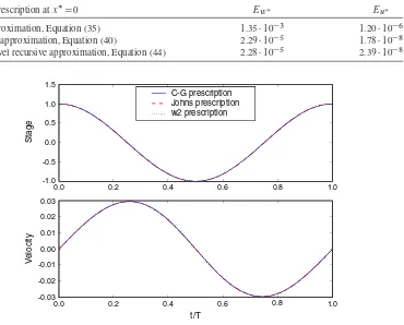
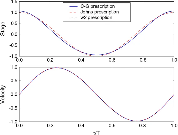
When the Johns approximation (35), the quadratic approximation (40), and the second level recursive approximation (44) are prescribed at positionx_{D0for timeton the intervalŒ0,T,} dis-crepancies between each of those approximations and the Carrier–Greenspan exact solution occur. If we discretize the time intervalŒ0,T_{into 1000 nodes, the average absolute discrepancy atxD0} for stagew_{and velocityuare as given in Table I. Those discrepancies are very small, but} obvi-ously the quadratic approximation (40) and the second level recursive approximation (44) result in much smaller discrepancies. The results for the quadratic approximation (40) and the results for the second level recursive approximation (44) are about the same order.

Figure 2 illustrates the Carrier–Greenspan exact solution, the Johns approximate solution, and the second level recursive approximation for stagew_{and velocityu at positionxD0for time}

t_{on the intervalŒ0,T. The discrepancies, in this case, are seen as negligible. We do not} graphi-cally show the results for the quadratic approximation because they are similar to the results for the second level recursive approximation.

Now, we investigate if the negligible discrepancy between the Carrier–Greenspan exact solution and the Johns approximate solution atx_{D0leads to a negligible discrepancy of any flow quantity}

Table I. Average absolute discrepancies (errors)Eatx_{D0when the setting of the first test case is taken.}

Here, the time intervalŒ0,T_{is discretized into 1000 nodes. SubscriptswanduofEdenote the average}

absolute discrepancy for stagew_{and velocityu, respectively.}

Stagewprescription atx_{D0 Ew Eu}

Johns approximation, Equation (35) 1.35103 _1.20106 Quadratic approximation, Equation (40) 2.29105 _1.78108 Second level recursive approximation, Equation (44) 2.28105 _2.39

108

C-G prescription Johns prescription w2 prescription

0.0 0.2 0.4 0.6 0.8 1.0

-1.0 -0.5 0.0 0.5 1.0 1.5

Stage

0.0 0.2 0.4 0.6 0.8 1.0

t/T -0.03

-0.02 -0.01 0.00 0.01 0.02 0.03

Velocity

Figure 2. Prescriptions forw_{andu atxD0. Here,LD50,000,h}

0D500,D1.0, andTD900.

‘C–G prescription’ stands for the Carrier–Greenspan exact prescription (18); ‘Johns prescription’ means the Johns prescription (35); ‘w2 prescription’ means the prescription ofw2that is the second level recursive

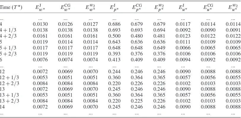
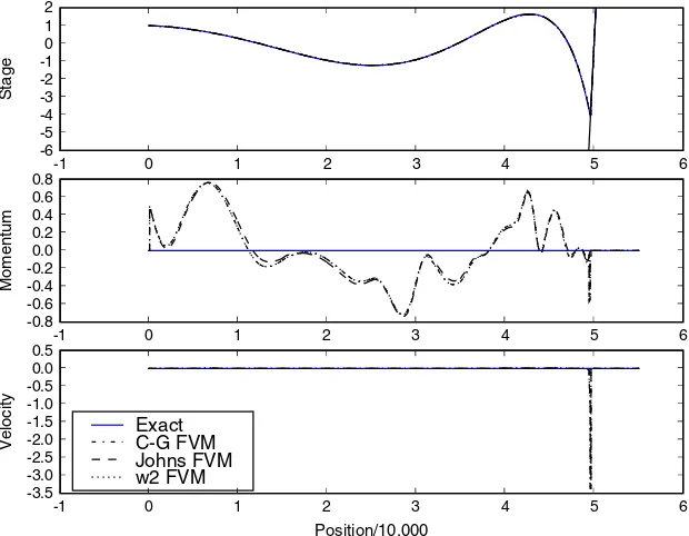
when those solutions atx_{D0are prescribed in numerical simulations to generate periodic waves.} We compare here the performance of the Johns approximate solution (35) and that of the second level recursive approximation (44). Starting from quiescent state, the numerical method generates a periodic solution after four periods of oscillation. The error comparison is presented in Table II. In general, the method with Carrier–Greenspan exact prescription results in smaller error. This is because the prescription discrepancy atx_{D0propagates towards the shoreline as the time evolves,} and consequently the error produced by the numerical method with the approximate prescription is larger than that produced by the numerical method with the exact prescription. However, we see that the discrepancies of the errors produced using the Johns prescription and Carrier–Greenspan exact prescription are small, as are the discrepancies of the errors produced using the second level recursive approximation and Carrier–Greenspan exact prescription. Figure 3 shows the stagew_, momentump_{, and velocity u at timetD14T. A large error in terms of the velocity occurs} around the wet/dry interface: This is called the wet/dry interface or wetting and drying problem. It should be stressed that this problem is caused by the inaccuracy of the numerical method that we use at the wet/dry interface and does not relate to whether the prescription applied in the numerical simulation is exact or approximate. Through more recent research, we are working on this wet/dry interface problem to get a more accurate resolution. Some authors, such as Bollermann, Kurganov, and Noelle [9], Briganti and Dodd [10], Brufau, Vázquez-Cendón, and García-Navarro [11], and Gallardo, Parés, and Castro [12], have also attempted to resolve this wet/dry interface problem.

It is worth questioning why the discrepancy of the solutions atx_{D0in this test case is negligible.} This error is due to the small magnitude of the amplitude factorA_{in this test case. Recall that the} amplitude factorA_{is found from the process of linearization of an equation discussed in} Subsec-tion 3.4. The linear approximaSubsec-tion matches exactly with the exact soluSubsec-tion whenA_D0. In addition, a small magnitude ofA_{leads to a small error of the linear approximation; a larger magnitude of}A results in a larger error of the linear approximation.

Recalling the specified values of the dimensional lengthL_{D50,000, dimensional heighth} 0D500,

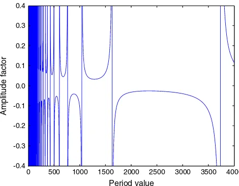
and dimensional amplitude_{D1.0, we can plot a graph relating the dimensional periodTand the} amplitude factorA_{as given in Figure 4 using Equation (37). The vertical lines in the figure are the} asymptotes, which are the singularities ofA, that is, the zeros of the denominator in Equation (37). ForT_{D900, the amplitude factor isAD 8.1810}3_.

Table II. ErrorsEfor various times. Here,L_D50,000,h

0D500,D1.0, andTD900. Subscriptsw,

p_{, anduofEdenote the error for stagew, momentump, and velocityu, respectively. Superscript}

J ofEdenotes that the computation uses the Johns prescription, whereas superscript CG denotes that the computation uses Carrier–Greenspan exact prescription, and superscriptw2denotes that the computation

uses ourw2approximate prescription.

Time.T_{/ E}J

4 0.0130 0.0126 0.0127 0.686 0.679 0.679 0.0117 0.0114 0.0114

4C1=3 0.0138 0.0138 0.0138 0.693 0.693 0.694 0.0092 0.0090 0.0091

4C2=3 0.0161 0.0161 0.0161 0.500 0.480 0.481 0.0123 0.0122 0.0122

5 0.0119 0.0114 0.0114 0.643 0.636 0.636 0.0111 0.0109 0.0109

5C1=3 0.0117 0.0117 0.0117 0.648 0.648 0.649 0.0066 0.0065 0.0065

5C2=3 0.0119 0.0119 0.0119 0.393 0.376 0.376 0.0106 0.0106 0.0106

6 0.0076 0.0074 0.0074 0.413 0.409 0.409 0.0094 0.0092 0.0092

... ... ... ... ... ... ... ... ... ...

12 0.0072 0.0069 0.0070 0.244 0.246 0.246 0.0090 0.0088 0.0088

12C1=3 0.0053 0.0051 0.0051 0.360 0.364 0.365 0.0057 0.0056 0.0055

12C2=3 0.0084 0.0084 0.0084 0.220 0.226 0.226 0.0102 0.0103 0.0103

13 0.0072 0.0069 0.0070 0.245 0.246 0.246 0.0090 0.0088 0.0088

13C1=3 0.0053 0.0051 0.0051 0.360 0.364 0.365 0.0057 0.0056 0.0055

13C2=3 0.0084 0.0084 0.0084 0.220 0.225 0.226 0.0102 0.0103 0.0103

14 0.0072 0.0069 0.0070 0.245 0.246 0.246 0.0090 0.0088 0.0088

-1 0 1 2 3 4 5 6 -6

-5 -4 -3 -2 -1 0 1 2

Stage

-1 0 1 2 3 4 5 6

-0.8 -0.6 -0.4 -0.2 0.0 0.2 0.4 0.6 0.8

Momentum

Exact C-G FVM Johns FVM w2 FVM

-1 0 1 2 3 4 5 6

Position/10,000

-3.5 -3.0 -2.5 -2.0 -1.5 -1.0 -0.5 0.0 0.5

Velocity

Figure 3. Solutions forw_{,p, anduattD14T. Here,LD50,000,h}

0D500,D1.0, andTD900.

‘Exact’ means the Carrier–Greenspan exact solution; ‘C–G FVM’ is the numerical solution by FVM with the exact prescription (18); ‘Johns FVM’ is the numerical solution by FVM with the Johns prescription (35); ‘w2 FVM’ is the numerical solution by FVM with the prescription ofw2that is the second level recursive

approximation (44).

0 200 400 600 800 1000 1200

Period value -0.10

-0.05 0.00 0.05 0.10

Amplitude factor

Figure 4. Relation of the dimensional periodT_{and the amplitude factor}A_{forLD50,000,h0D500, and}

_{D1.0. The vertical lines are asymptotes.}

Roughly speaking, using the specified values of the dimensional lengthL_{, dimensional height}

h

0, and dimensional amplitudein this first test case, the Johns approximate solution (found by

involving a linearization of an equation) atx_{D0is accurate on some intervals of the dimensional} period T_{, such asŒ800,1000, where all points in this interval are far enough from asymptotes.} This is illustrated in Figure 4 in which the tangent lines on the intervalŒ800,1000, especially for points aroundT_{D900, are almost horizontal.}

Using the same values of the dimensional length L_{, dimensional height h}

0, and dimensional

approximate and the exact solutions atx_{D0, as shown in Figure 5. Now, we haveAD5.2610}2_.

When we discretize the time intervalŒ0,T_{into 1000 nodes, the average absolute discrepancy at}

x_{D0for stagewand velocityuare5.6510}2_and1.30

104_{, respectively, for the Johns}

approx-imate solution, and3.16103 _and6.83

106_{, respectively, for our second level approximation.}

These discrepancies for the Johns approximate solution are still relatively small. Unfortunately, if we take a larger value ofT_{closer to the asymptote lying on the intervalŒ1000,1200to get a larger} value ofA_{, the Jacobian}@ .x,t / =@ .,/may vanish in >0, that is, a breaking wave occurs. The vanishing of the Jacobian@ .x,t / =@ .,/can be verified analytically from Equations (11), (15), (16), and (17).

4.2. Second test case: the Johns prescription fails

In this subsection, we present a test case where the Johns prescription (35) fails to accurately approx-imate the Carrier–Greenspan exact solution atx_{D0. We consider a spatial domain given by the} interval [50, 65,050] discretized into 651 cells. The dimensional lengthL_{D50,000, dimensional} heighth

0D500, and dimensional periodTD3600are taken. We fixD5.0in this test case. We

consider these values in order to get a larger value of amplitude factorA_{than the value of}A_{in the} first test case and that the Jacobian@ .x,t / =@ .,/does not vanish in >0. Hence, the error of the Johns prescription (35) in this test case is larger than that in the first test case.

The setting here implies that the shoreline position at any time lies on the interval [38,745.65, 61,254.35] sinceA_D 2.25101 _{and that no breaking wave occurs. In a half of the period of}

oscillation, the shoreline travels a distance more than22.5103. This distance is more than 27 times the distance traveled by the shoreline in the first test case. Recalling the specified values of the dimensional lengthL_{, dimensional heighth}

0, and dimensional amplitude, we plot the relation

between the dimensional periodT_{and the amplitude factorAin Figure 6.}

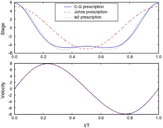
When the Johns approximation (35), the quadratic approximation (40), and the second level recursive approximation (44) are prescribed at positionx_{D0for timeton the intervalŒ0,T,} dis-crepancies between each of those approximations and the Carrier–Greenspan exact solution occur. Discretizing the time intervalŒ0,T_{into 1000 nodes, we obtain that the average absolute} discrep-ancy atx_{D0for stagewand velocity u are as given in Table III. We see that the quadratic}

C-G prescription Johns prescription w2 prescription

0.0 0.2 0.4 0.6

-1.0 -0.5 0.0 0.5 1.0 1.5

Stage

0.0 0.2 0.4 0.6

0.8 1.0

0.8 1.0

t/T

-1.0 -0.5 0.0 0.5 1.0

Velocity

Figure 5. Solutions forw _{andu at xD0. Here,LD50,000,h}

0D500,D1.0, andTD1020.

‘C–G prescription’ stands for the Carrier–Greenspan exact prescription (18); ‘Johns prescription’ means the Johns prescription (35); ‘w2 prescription’ means the prescription ofw2that is the second level recursive

0 500 1000 1500 2000 2500 3000 3500 4000 Period value

-0.4 -0.3 -0.2 -0.1 0.0 0.1 0.2 0.3 0.4

Amplitude factor

Figure 6. Relation of the dimensional periodT_{and the amplitude factorAforLD50,000,h}

0D500, and

_{D5.0. The vertical lines are asymptotes.}

Table III. Average absolute discrepancies (errors)Eatx_{D0when the setting of the second test case is}

taken. Here the time intervalŒ0,T_{is discretized into 1000 nodes. SubscriptswanduofEdenote the}

average absolute discrepancy for stagew_{and velocityu, respectively.}

Stagewprescription atx_{D0 E}

w E_u

Johns approximation, Equation (35) 1.83 2.69102 Quadratic approximation, Equation (40) 3.19101 _4.26

103

Second level recursive approximation, Equation (44) 2.88101 _3.85103

approximation (40) and the second level recursive approximation (44) results in much smaller dis-crepancies than the disdis-crepancies that result from the Johns approximate solution (35). The results for the quadratic approximation (40) and the results for the second level recursive approximation (44) are again about the same order.

Figure 7 illustrates the Carrier–Greenspan exact solution, the Johns approximate solution, and the second level recursive approximation for stagew _{and velocityu at positionxD0for timet} on the intervalŒ0,T_{. The discrepancies that result from the Johns approximate solution are now} large, whereas the discrepancies from the second level recursive approximation are much smaller. We do not graphically show the results for the quadratic approximation because they are similar to the results for the second level recursive approximation.

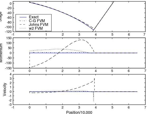
The method with the Johns prescription produces very large errors, as shown in Table IV. Large errors can also be observed graphically for the stagew_{, momentump, and velocityu at time}

t_{D14T, as illustrated in Figure 8. A magnification of Figure 8, depicting the stagewat cells} around the wet/dry interfaces on the interval [38,400, 39,400], is shown in Figure 9. Notice that in Figure 9, the horizontal and the vertical distances from the wet/dry interface for the Carrier– Greenspan exact solution to the wet/dry interface for the numerical solution generated using the Johns prescription are about500and5, respectively.

In this test case, the linearization of Equation (22) done by Johns [5] results in a poor approx-imation of the exact solution atx_{D0. This poor approximation then leads to a very large error} when it is prescribed in place of the Carrier–Greenspan exact solution atx_{D0to generate periodic} waves in the numerical simulation. According to the simulation results, our second level recursive approximation (44) indeed produces smaller errors than the Johns approximate solution (35).

5. RATE OF CONVERGENCE

C-G prescription

‘C–G prescription’ stands for the Carrier–Greenspan exact prescription (18); ‘Johns prescription’ means Johns prescription (35); ‘w2 prescription’ means the prescription ofw2that is the second level recursive

approximation (44).

Table IV. ErrorsEfor various times. Here,L_D50,000,h

0D500,D5.0, andTD3600. Subscriptsw,

p_{, anduofEdenote the error for stagew, momentump, and velocityu, respectively. Superscript}

J ofEdenotes that the computation uses the Johns prescription, whereas superscript CG denotes that the computation uses Carrier–Greenspan exact prescription, and superscriptw2denotes that the computation

uses ourw2approximate prescription.

Time.T_{/ E}J

13 0.999 0.048 0.238 50.077 2.459 15.752 0.376 0.014 0.069

13C1=6 1.083 0.065 0.262 46.711 0.902 5.305 0.459 0.009 0.090

13C2=6 2.187 0.030 0.320 22.999 3.626 8.844 0.266 0.046 0.078

13C3=6 0.841 0.041 0.240 47.976 3.038 15.831 0.373 0.017 0.071

13C4=6 0.872 0.066 0.218 42.886 1.075 5.827 0.438 0.066 0.147

13C5=6 2.124 0.044 0.276 29.172 3.411 8.404 0.288 0.139 0.147

14 1.001 0.048 0.237 50.230 2.433 15.712 0.377 0.014 0.069

... ... ... ... ... ... ... ... ... ...

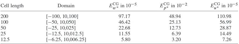
We expect that the numerical method leads to a first order of convergence because we take a first order discretization at the prescribed cell. Because of the wet/dry interface problem, the expected rate of convergence is not achieved, as can be observed in Table V. However, if we truncate the spatial domain in such a way that the computation does not involve the wet/dry interface problem, the numerical method we use indeed results in a first order of convergence, as shown in Table VI. This first order of convergence is observed because the errors produced by the numerical method are halved as the cell length is halved.

Exact C-G FVM Johns FVM w2 FVM

-1 0 1 2 3 4 5 6 7

-120 -100 -80 -60 -40 -20 0

Stage

-1 0 1 2 3 4 5

-150 -100 -50 0 50 100 150

Momentum

-1 0 1 2 3 4 5

6 7

6 7

Position/10,000 -3

-2 -1 0 1 2 3 4

Velocity

Figure 8. Solutions for w_{,p, andu at tD14T. Here, L D50,000, h}

0 D500, D5.0, and

T_{D3600. ‘Exact’ means the Carrier–Greenspan exact solution; ‘C–G FVM’ is the numerical solution by}

FVM with the exact prescription (18); ‘Johns FVM’ is the numerical solution by FVM with the Johns pre-scription (35); ‘w2 FVM’ is the numerical solution by FVM with the prepre-scription ofw2that is the second

level recursive approximation (44).

Exact C-G FVM Johns FVM w2 FVM

3.82 3.84 3.86 3.88 3.90 3.92 3.94 Position/10,000

-114 -112 -110 -108 -106 -104 -102 -100

Stage

Figure 9. A magnification of Figure 8 for w _{on the interval [38,400, 39,400]. Here, t D 14T,}

L_{D50,000, h}

0D500,D5.0, andTD3600. ‘Exact’ means the Carrier–Greenspan exact solution;

‘C–G FVM’ is the numerical solution by FVM with the exact prescription; ‘Johns FVM’ is the numeri-cal solution by FVM with the Johns prescription; ‘w2 FVM’ is the numerinumeri-cal solution by FVM with the

prescription ofw2that is the second level recursive approximation.

6. CONCLUSION

Table V. ErrorsE for various uniform cell lengths (x) of spatial discretization. Here,L_D50,000,

h

0D500,D1.0, andTD900. Subscriptsw,p, anduofEdenote the error for stagew, momentum

p_{, and velocityu, respectively. Superscript CG ofEdenotes that the computation uses Carrier–Greenspan}

exact prescription. Domain means the interval of spatial domain to be considered and discretized. The errors are computed att_D14T_.

Cell length Domain ECG

win103 E_pCGin102 E_uCG in104

200 [100, 55,100] 23.84 88.19 254.05

100 [50, 55,050] 6.95 24.64 88.12

50 [25, 55,025] 2.13 13.19 35.25

25 [12.5, 55,012.5] 1.36 9.36 8.42

12.5 [6.25, 55,006.25] 1.26 7.24 6.23

Table VI. ErrorsE for various uniform cell lengths (x) of spatial discretization. Here, L_D50,000,

h

0D500,D1.0, andTD900. Subscriptsw,p, anduofEdenote the error for stagew, momentum

p_{, and velocityu, respectively. Superscript CG ofEdenotes that the computation uses Carrier–Greenspan}

exact prescription. Domain means the interval of spatial domain to be considered and discretized. The errors are computed att_DT_.

Cell length Domain ECG win10

5 _ECG

p in10

2 _ECG

u in10

5

200 [100, 10,100] 97.17 48.94 110.98

100 [50, 10,050] 46.42 25.13 56.99

50 [25, 10,025] 22.68 12.73 28.87

25 [12.5, 10,012.5] 11.55 6.39 14.49

12.5 [6.25, 10,006.25] 5.80 3.20 7.26

periodic solution, which are more accurate than the Johns approximate solution at the zero point of the spatial domain. In addition, results of a finite volume method with the approximate prescriptions applied at the fixed boundary to generate periodic waves on a sloping beach have been compared with those of the same method with the Carrier–Greenspan exact prescription.

We have found that if the discrepancy between the approximate and the exact prescriptions is negligible, the errors of both numerical solutions are similar. If the discrepancy is very large, the error of the numerical solution with the approximate prescription is much larger than that of the numerical solution with the exact prescription. This means that the prescription at the fixed bound-ary significantly affects the error of the numerical solution. Therefore, we suggest that the exact, instead of the approximate prescription, should be applied when the Carrier–Greenspan periodic waves are used to assess the performance of a numerical method.

However, if an explicit formulation of the stage at the zero point of the spatial domain is needed, such as for developing a numerical technique, an approximation of it can be taken. We can take either the approximate solution of Johns, the quadratic approximation, the second level recursive approximation, or another approximation as long as it is guaranteed that the error produced at the zero point of the spatial domain is negligible.

ACKNOWLEDGEMENTS

We thank the reviewers for their insightful and constructive comments, which have significantly improved the quality of the manuscript. For helpful discussions that improved this writing technically, we thank Nick Gouth at the Mathematical Sciences Institute, The Australian National University (ANU). Some discussions with Christopher Zoppou at the ANU are also acknowledged. The work of Sudi Mungkasi was supported by ANU PhD and ANU Tuition Scholarships.

REFERENCES

1. Carrier GF, Greenspan HP. Water waves of finite amplitude on a sloping beach.Journal of Fluid Mechanics1958;

4_{(1):97–109.}

3. Brocchini M, Svendsen IA, Prasad RS, Bellotti G. A comparison of two different types of shoreline boundary conditions.Computer Methods in Applied Mechanics and Engineering2002;191_{(39–40):4475–4496.}

4. Dietrich JC, Kolar RL, Luettich RA. Assessment ofADCIRC’s wetting and drying algorithm. InProceedings of the 15th International Conference on Computational Methods in Water Resources (CMWR XV), Chapel Hill, 13–17 June 2004, Vol. 2, Miller CT, Farthing MW, Gray WG, Pinder GF (eds). Elsevier: Amsterdam, 2004; 1767–1778. 5. Johns B. Numerical integration of the shallow water equations over a sloping shelf. International Journal for

Numerical Methods in Fluids1982;2_{(3):253–261.}

6. Sidén GLD, Lynch DR. Wave equation hydrodynamics on deforming elements.International Journal for Numerical Methods in Fluids1988;8_{(9):1071–1093.}

7. Mungkasi S, Roberts SG. On the best quantity reconstructions for a well balanced finite volume method used to solve the shallow water wave equations with a wet/dry interface.The Australian and New Zealand Industrial and Applied Mathematics Journal2010;51_{(EMAC2009):C48–C65.}

8. Kurganov A, Noelle S, Petrova G. Semidiscrete central-upwind schemes for hyperbolic conservation laws and Hamilton–Jacobi equations.SIAM Journal on Scientific Computing2001;23_{(3):707–740.}

9. Bollermann A, Kurganov A, Noelle N. A well-balanced reconstruction for wetting/drying fronts.IGPM Report2010;

313_:1–18.

10. Briganti R, Dodd N. Shoreline motion in nonlinear shallow water coastal models. Coastal Engineering2009;

56_{(5–6):495–505.}

11. Brufau P, Vázquez-Cendón ME, García-Navarro P. A numerical model for the flooding and drying of irregular domains.International Journal for Numerical Methods in Fluids2002;39_{(3):247–275.}

12. Gallardo JM, Parés C, Castro M. On a well-balanced high-order finite volume scheme for shallow water equations with topography and dry areas.Journal of Computational Physics2007;227_{(1):574–601.}

13. Audusse E, Bouchut F, Bristeau MO, Klein R, Perthame B. A fast and stable well-balanced scheme with hydrostatic reconstruction for shallow water flows.SIAM Journal on Scientific Computing2004;25_{(6):2050–2065.}