•DownloadRandRpackagesforyourplatform •WorkwithRwithinyourfilestructure
•Enterdatafromthekeyboardandfromexternalfiles •Determineandassignmodes,classes,andtypesofobjects •DocalculationsusingthecomputationaltoolsinR
For your convenience Apress has placed some of the front
matter material after the index. Please use the Bookmarks
and Contents at a Glance links to access them.
Contents at a Glance
About the Author ...
xv
About the Technical Reviewer ...
xvii
Acknowledgments ...
xix
Introduction ...
xxi
Part 1: R Basics
■
...
1
Chapter 1: Downloading R and Setting Up a File System
■
...
3
Chapter 2: The R Prompt
■
...
9
Chapter 3: Assignments and Operators
■
...
11
Part 2: Kinds of Objects
■
...
23
Chapter 4: Modes of Objects
■
...
25
Chapter 5: Classes of Objects
■
...
37
Part 3: Functions
■
...
57
Chapter 6: Packaged Functions
■
...
59
Chapter 7: User-Created Functions
■
...
65
vi
Part 4: Inputting and Creating Data, Outputting Data
■
and Output, and Manipulating Objects ...
77
Chapter 9: Importing and Creating Data
■
...
79
Chapter 10: Exporting from R
■
...
95
Chapter 11: Descriptive Functions and Manipulating Objects
■
....
105
Part 5: Flow Control
■
...
127
Chapter 12: Flow Control
■
...
129
Chapter 13: Examples of Flow Control
■
...
133
Chapter 14: The Functions ifelse( ) and switch( )
■
...
145
Part 6: Some Common Functions, Packages, and
■
Techniques ...
151
Chapter 15: Some Common Functions
■
...
153
Chapter 16: The Packages base, stats, and graphics
■
...
163
Chapter 17: Tricks of the Trade
■
...
189
Introduction
R is a programming language that provides the user with powerful data and graphical analysis options. R is both flexible and broad. From tasks as simple as adding two numbers to tasks as complex as fitting an ARIMA model, R is capable of crunching the numbers.
The purpose of R Quick Syntax Reference is to provide the reader with the basic syntax of R. Often an R user gets stuck if, for example, a mode is incorrect or a logical test does not work. Because the full spectrum of R packages uses the same fairly simple syntax, R Quick Syntax Reference provides the reader with the necessary information to get unstuck and run and create all R functions and code.
The R language is based on the language S, a high-level programming language developed mainly by Richard A. Becker, John M. Chambers, and Allan R. Wilks in the AT&T laboratories in 1975. The R version of the language first became available in 1993 and was developed by Ross Ihaka and Robert Gentleman at the University of Auckland, New Zealand.
R is open source and is a GNU project. As open-source code, the R language is free and constantly being improved. The R Development Core Team currently does the development. Packages for specific analysis techniques are added often. At the present time, there are 4,986 packages available in R. Most users will use only a few packages. Although GUI versions of R are available, we discuss using R at the command prompt in
R Quick Syntax Reference.
This book is about the S3 version of R—S3 standing for the third version of S, the commercial program on which R is based. The developers of R have a new version, S4—the fourth version of S—running concurrently with S3. Even though version S4 is quite different from S3, it is necessary to know the syntax of S3 in order to use S4. And S3 remains a powerful, flexible language in its own right—hence, this book.
Part I covers the basics of R. Chapter 1 describes how to download and install R for the Windows, Mac, and Linux operating systems and also how to download packages. Because keeping separate folders for different projects is very useful, Chapter 1 gives instructions for running R from different folders. It also gives the methods for updating the R program itself.
Chapter 2 introduces the R prompt, gives a sample calculation, and describes the three parts of R—objects, operators, and assignments. Chapter 3 covers the assignment of names to objects, demonstrates the ls() function that allows you to see the objects in a folder, and discusses the operators in R.
xxii
Part III covers functions. Chapter 6 starts with a list of the 30 default packages in R and follows with instructions on how to use functions. Because packaged functions all have help pages, the chapter provides instructions on how to access and use the help page of a function. Chapter 7 describes how to create a function. Chapter 8 explains how to run a function—with a detailed approach to the argument list.
Part IV focuses on importing and exporting data in R and methods for creating and manipulating some kinds of object. Chapter 9 describes several methods for importing data, gives a number of functions to create data objects, and discusses some random-number generators. Chapter 10 gives several methods for exporting from R. Chapter 11 gives a number of functions that operate on objects—to bind objects together, to find descriptive qualities of an object, to assign qualities to an object, to aggregate an object in some way, or to apply functions to portions of an object.
Part V covers flow conditioning commands and functions. Chapter 12 presents the flow conditioning statements, and Chapter 13 supplies examples of them. Chapter 14 describes the two flow conditioning functions and gives examples.
R Basics
Part I introduces you to the basics of the R language.
To use R, you must first download the program from the Internet. Chapter 1 describes how to install R on the Windows, OS X, and Linux operating systems. It also describes how to install and update packages and how to update R and use R within a file system.
Once you’ve installed and opened R, you are faced with an R prompt and little else. Chapter 2 presents the parts of R (objects, operators, and assignments), the R prompt, and an example of using R as a calculator from the R prompt.
3
Downloading R and Setting
Up a File System
The first step in using R is to download R from the Internet. R can be downloaded for the modern operating systems Windows, OS X, and Linux. In this chapter, you will learn how to download and install R and the 30 basic packages as well as how to install other packages and update R. You will also learn how to use R in individual folders within the file system of the computer.
Downloading R
You can download R from the web site of the Comprehensive R Archive Network (CRAN). CRAN updates the installation process from time to time; however, the instructions in this book are for the current steps at time of publication. CRAN provides instructions on the web site if the process has changed.
Begin the download process by going to the web site http://cran.r-project.org. At the web site, links to current versions for Windows, OS X, and Linux are listed at the top of the opening window. Select the appropriate link.
Windows
On the page that opens with the Windows link, select the link base, which is the top link. In the next window, click on the download link for the given Windows version.
(Currently, the link is Download R 3.0.2 for Windows.) If R has not already been installed on the computer, the downloader will create a default folder in the Documents folder to hold R files. Unless there is a reason to change the folder name or location, accept the default. R will begin to download.
The installation wizard will open. The installation process steps through several pages. On the first page, read the GNU GENERAL PUBLIC LICENSE; then click on Next. For the rest of the pages, accepting the defaults on each page is fine, so click on Next on each page.
At the page of additional choices, click on Next, and the program will begin to install. When the installation is finished, click on Finish to complete the installation. The program and the 30 base packages are now installed. An icon for R will be on the computer desktop and, for Windows 8, in the charms. To run R, click on the icon or charm.
OS X
On the page that opens from the OS X link, first read the section under R for Mac OS X. The R project gives the advice to check the files for viruses and other problems.
Under Files: there are two package choices: the current version and latest version. Selecting the current version (the .pkg link, currently R-3.0.2.pkg) will download both packages. When the packages have finished downloading, open the download box on the icon bar (the yellow and brown box) or the downloads folder under the username in Finder.
Select an R version in the download box. Opening the version will open the installer. With the installer open, click on Continue to go to the next page of the installer. Read the message from CRAN; then click Continue. Again, read the message from CRAN; then click Continue.
On the next page, you will find the license. After reading the license, click Agree to download R. On the next page, select either of the choices; then click on Continue. (The Continue button will not light up until a choice is made.)
On the next page, select Install. The installation program will ask for a password. After you have entered a password, the installation will begin. When the installation is finished, click on Close. R will now be in the applications folder and on the dock and the 30 base packages will be loaded. Select R on the dock or in the applications folder to start R.
Linux
At the CRAN site, CRAN provides source code for R for the Linux distributions Debian, Red Hat, Suse, and Ubuntu. The developers state that R is available through the package management system for most distributions of Linux.
If the command line version of R is not available using the package management system, installing R directly from the terminal is an option. At http://cran.r-project.org/ bin/linux/distribution, where distribution is Debian, Suse, or Ubuntu, you can find instructions for installing R from the terminal command prompt under the ReadMe files.
For Red Hat, http://cran.r-project.org/bin/linux/redhat, there is no ReadMe
5
Installing and Updating Packages
When initially installed, R comes with 30 packages. Often the user will want to use the power of the many other packages available in R. Installing and updating a package is straightforward.
For any of the operating systems, if the name of a package is known, typing
install.packages("package name")
at the R command prompt, where package name is the name of the package, will install the package. To update packages, typing
update.packages()
at the R command prompt will find those packages with updates and update the packages. To see which packages are already installed on the computer, enter
installed.packages()
at the R prompt.
If the name of the package is not known (also for known names), using the installer for the operating systems Windows and OS X is easy. For Linux, instructions can be found at the CRAN web site, http://cran.r-project.org. Here you can find instructions for Windows and OS X.
Windows
To install a package in Windows not using the command line, start by opening R. On the menu bar at the top of the screen, select Packages. A menu will drop down. Select Install package (s). . . . Either the CRAN mirror window or the Packages window will come up. If the CRAN mirror window comes up, select a close mirror and click OK, which will bring up the Packages window.
The Packages window consists of a list of all of the available packages. Scroll down the list to find the package(s) you wish to install and select the package(s). Click on OK to begin the installation. As the installation proceeds, the steps of the installation will scroll on the R console. When the R prompt returns to the screen, the installation is complete.
OS X
To install packages in OS X, start by opening R. On the menu bar at the top of the screen, select Packages & Data. From the drop-down menu, select Package Installer, which brings up the R Package Installer. Click on Get List for a full list of packages or use the Package Search option to search for a package. Under either option, select the package(s) to be installed from the list.
Below the list of packages are choices for the location to put the packages. Hover over the list of location options for more information. Usually, one of the first two options will be correct. To the right of the location options are the Install Selected and Update All buttons. Before clicking on Install Selected, check the Install Dependencies box to make sure that any necessary packages are installed. Click on Install Selected to start the installation process. The selected packages will install.
To update packages, select Packages & Data from the menu bar at the top of the screen. From the drop-down menu, select Package Installer, which opens up the R Package Installer. At the bottom right of the Installer, select Update All and follow instructions.
Updating R
Since CRAN does not provide automatic updates for R, you must update it manually. The processes for Windows and OS X are easy. For the Linux distributions Debian, Suse, and Ubuntu, instructions can be found in the ReadMe files at http://cran.r-project/bin/ linux/distribution, where distribution is either Debian, Suse, or Ubuntu. For Red Hat Linux, look elsewhere on the CRAN web site.
Windows
The first step in updating R in Windows is to open R and install the package installr if the package has not already been installed. Next, use the function library to provide access to
installr. Type
library(installr)
at the command prompt and press enter. Then, to update R, type
updateR()
at the command prompt and press enter. R will either do an update or give a message that the program is up-to-date and return False.
7
OS X
The first step in updating R in OS X is to open R and select R from the menu bar at the top of the page. To run the updater, select Check for R Updates in the drop-down menu under R and follow instructions.
Using R in Separate Folders
Separate workspace images for R can be maintained in separate folders for Windows, OS X, and Linux. This property of R is very handy for using R on separate projects. While the process of opening R in a given folder varies by the operating system, once in a folder, saving the workspace image is straightforward. When closing an R session, the program asks if the user would like to save the workspace image. If Yes is selected, then .RData and
.Rhistory (.Rapp.history for OS X) files are saved in the current directory. (For OS X, the files are hidden, but the files are there.)
The .RData file contains the objects that were in R at the beginning of the session plus any objects that were added during the session minus any objects that were erased during the session. The .Rhistory (.Rapp.history for OS X) file contains the history of the lines input at the R console. By default, all lines up to the last 512 lines are saved in Windows. For OS X and Linux, the default is 250 lines. Access to the lines carries over from session to session if the history is saved.
Windows
To initially set up R in a folder, open R at the desktop. (Click on the R icon on the desktop or click on R in the list of programs or, in Windows 8, the list of charms.) Select File on the menu bar at the top of the screen. From the drop-down menu, select Change dir. . .. The
Browse to folder window will open. Navigate to the folder of choice.
When exiting R, save the workspace image and R will create .RData and .Rhistory
files in the folder. The .RData file will have a blue R icon associated with the file. In the future, going to the folder and clicking on the R icon will open R and the history and objects saved within the folder will be present.
As a note for the initial setup, any objects in the desktop R will still be in R when the folder is changed. You can easily remove the objects. Type rm(list=ls()) at the command prompt to remove all objects from the folder.
OS X
To open R using the terminal, open the terminal (located under Applications/ Utilities in Finder.) and type
open -a R folder
where folder is the location of the folder. R will open in the folder using the .RData and
.Rapp.history files for that folder.
Linux
9
The R Prompt
This chapter covers the R prompt. It starts with descriptions of the three parts of R: objects, operators, and assignments. It continues with a discussion of working with the R prompt, followed by an example of doing a calculation at the R prompt.
In Windows and OS X, R runs in GUIs: RGUI in Windows and R.app GUI in OS X. Both RGUI and R.app GUI open an R Console and run from the R prompt in the R Console. GUIs are available in Linux, but this book covers only running R from the terminal window R prompt.
The Three Parts of R: Objects, Operators, and
Assignments
There are basically three parts of R: objects, operators, and assignments.
Objects contain information and can be data, functions, or the results of functions. Objects always have a name. Users create some objects, which are automatically saved on creation. Other objects are functions and datasets contained in the packages of R.
Operators manipulate the objects, numbers, strings, and/or logical variables. For example, entering a = 2*bat the R prompt would multiply bby two and assign the result to a. The objects
aandbare numeric objects and *is the multiplication operator. The equal sign makes an assignment of two timesbtoa. Assignments assign an expression to an object. Expressions
consist of objects, numbers, logical variables, and/or strings, which are operated on by operators.
The R Prompt
All of R flows from the R prompt. R is essentially the running of functions and the doing of calculations. Functions and calculations can be run at the R prompt with or without an assignment to an object. Functions and calculations can also be run as part of a function, but everything starts at the R prompt.
Using R from the R prompt may seem daunting at first. R opens with some script, and then a lonely little greater-than sign (>) is the R prompt. The opening script gives the R version number and some other information about the program, including the fact that the program runs with no warranty.
R remembers every line that is entered into the program, up to a set number of lines. A very handy side of R is that the up and down arrows on the keyboard will step through the lines. You only need to enter an expression once. Corrections to expressions are easy to do without typing the entire expression again.
To close R, enter q( ) at the R prompt or, for Windows and OS X, close the window. R will close with the option to save the workspace. In Linux, if the terminal window is closed without using q( ), the current workspace will be lost.
The workspace consists of any objects present in R at the time the program is closed and the current history. Closing R without saving the workspace will result in reverting to the workspace present at the time the R session started.
An Example of a Calculation
The simplest use of R is as a calculator. The following calculation was done from the R prompt. There is no assignment in the calculation, so the result is returned on the screen.
> (1 + 3 + 7)/5 [1] 2.2
>
11
Assignments and Operators
R works with objects. Objects can include vectors, matrices, functions, the results from a function, or a number of other kinds of objects. Objects make working with information easier. This chapter covers assigning names to objects, listing and removing objects, and object operations. Part II (Chapters 4 and 5) covers the possible forms of objects.
Some objects come with the packages in R. Other objects are user-created. User-created objects have names that are assigned by the user. Knowing how to create, list, and remove user-created objects is basic to R.
Types of Assignment
Names in R must begin with a letter or a period, cannot have breaks, and can contain letters, numeric digits, periods, and underscores. The names that begin with a period are hidden and are used by R for startup defaults, the random seed, and other such things. The indexing symbols [],[[]],$, and @ have special meanings with regard to R names, as explained the “Subscripting Operators” section of this chapter.
R originally used five types of assignment, four of which are still current. The four types are
a <- b,
which assigns b to a,
a -> b,
which assigns a to b,
a <<- b,
which assigns b to a and can be used inside a function to bring the assignment up to the workspace level, and
a ->> b,
Recently, the developers at R have included the more standard
a = b,
which assigns b to a. While any of the types of assignment can be used, the use of the equal sign is easiest to type.
When R makes an assignment, the name is automatically saved in the workspace. Note that no warning is given if the assigned name already exists. The assignment will overwrite the object in the workspace with the assigned object.
R is interesting in that a function of an object can be assigned to the original object. For example,
a = 2*a,
where the object a is replaced by the original a times two.
For more information about assignment operators, enter ?“Assignment Operators”
at the R prompt.
Example of Three Types of Assignment
An example of some of the types of assignment follows. Three objects are created: abc,
bcd, and cde. You create the objects by assigning sequences to the objects. The sequences are generated when you put a colon between two integers, which creates a sequence of integers starting with the first integer and ending with the second integer.
To show that the objects actually contain the assigned sequence, the contents of the three objects are displayed below. Note that entering the name of an object at the R prompt will always display the contents of the object. The [1] refers to the first element of the objects.
> abc = 1:10
> abc
[1] 1 2 3 4 5 6 7 8 9 10
> bcd <- 11:20
> bcd
[1] 11 12 13 14 15 16 17 18 19 20
> 21:30 -> cde
> cde
[1] 21 22 23 24 25 26 27 28 29 30
13
The ls( ) and rm( ) Functions
To see the objects present in the workspace, use the function ls(). Entering ls() at the R prompt for the above example gives
> ls()
[1] "abc" "bcd" "cde" >,
which are the three objects created above.
Although functions are covered in detail in Part III, one interesting property of functions to note here is they can have arguments that the user enters. Two of the possible arguments for ls() are pattern and all.names.
The first argument is entered as pattern = “a string”, where “a string” is any part of an object name. For example, in the above workspace, searching for those objects containing bc in the name gives abc and bcd, that is
> ls(pattern="bc") [1] "abc" "bcd"
The argument pattern can be reduced to pat, as in ls(pat=“bc”). The shortening of arguments of functions is a property of R. All arguments in R can be reduced to the shortest unique form, but they are usually given in the full form in manuals.
The second argument is all.names=, which can equal TRUE or FALSE. If set to TRUE, the all.names argument instructs R to list all of the files in the workspace, including those that begin with a period. FALSE is the default value and does not need to be entered. For the example workspace above, setting all.names equal to TRUE gives
> ls(all.n=T)
[1] ".commander.done" ".First" ".Random.seed" ".Traceback" [5] "abc" "bcd" "cde"
.
The [1] refers to “.commander.done” since “commander.done” is the first element of the vector, and the [5] refers to “abc” since “abc” is the fifth element of the vector. In R, if the elements of a vector have not been given a name, the convention for listing the elements is to show the index of the first element in each line of the lines of listed elements.
The function rm() can be used to remove objects from the workspace. For rm(), the names of the objects to be deleted are put within the parentheses and separated by commas. For example,
rm(a,b,c)
will remove objects a, b, and c. To remove all objects,
rm(list=ls())
works.
Operators
Operators operate on objects. Operators can be logical, arithmetic, matrix, relational, or subscripting, or they may have a special meaning. Each of the types of operators is described here.
For operators, elementwise refers to performing the operation on each element of an object or paired elements for two objects. If two objects do not have the same dimensions, the operator will cycle the smaller object against the larger object. The cycling proceeds through each dimension. For example, for matrices the first dimension is the rows and the second dimension is the columns, so the cycling is down rows starting with the first column.
The letters NA are used to indicate that an element is missing data. Most operators have rules for dealing with missing data and may return an NA if data is missing.
CRAN gives a help page of information about operation precedence. Enter
??“Operator Syntax and Precedence” at the R prompt to see the page.
Logical Operators and Functions
Logical operators return the values TRUE, FALSE, or NA, where NA refers to a missing value. The logical operators are the not operator, two or operators, two and operators, the
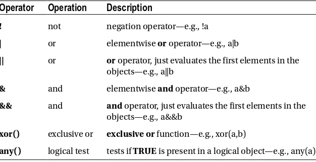
exclusive or function (which is a function that acts as an operator), and the any function (which is a function that operates on a logical object). For logical operators, if the two objects do not have the same dimensions, the number of elements in the larger object must be a multiple of the number of elements in the smaller object for cycling to occur. The logical operators and two logical functions are listed in Table 3-1.
Table 3-1. The Logical Operators and Functions
Operator
Operation
Description
! not negation operator—e.g., !a
| or elementwise or operator—e.g., a|b
|| or or operator, just evaluates the first elements in the objects—e.g., a||b
& and elementwise and operator—e.g., a&b
&& and and operator, just evaluates the first elements in the objects—e.g., a&&b
xor() exclusive or exclusive or function—e.g., xor(a,b)
any() logical test tests if TRUE is present in a logical object—e.g., any(a)
15
The negation operator changes TRUE to FALSE and FALSE to TRUE in a logical object. The operator | compares the two objects elementwise and, for each pair of elements, returns TRUE if TRUE is present, and FALSE otherwise. The operator ||
compares the first element of the first object to the first element of the second object and returns TRUE if TRUE is present, or FALSE otherwise.
The operator & compares two objects elementwise and, for each pair of elements, returns TRUE if both elements are TRUE, and FALSE otherwise. The operator &&
compares the first element of the first object to the first element of the second object and returns TRUE if the first elements are both TRUE, otherwise FALSE.
The xor() function compares objects elementwise and returns TRUE if the paired elements are different and FALSE if the paired elements are the same.
For a logical vector or a vector that can be coerced to logical, the function any() will return TRUE if any of the elements are TRUE, and FALSE otherwise.
For more information about the logical operators, the CRAN help pages for logical operators can be found by entering ??“logical operators” at the R prompt. The help page for any() can be accessed by entering ?any at the R prompt.
Arithmetic Operators
Arithmetic operators can have numeric operands or operands that can be coerced to numeric. For example, for logical objects TRUE coerces to 1 and FALSE coerces to 0. For some types of objects, specific operators have a different meaning, but those types of objects will not be covered in this chapter.
Arithmetic expressions are evaluated elementwise. If the number of elements is not the same between the objects in an expression, the smaller object cycles through the larger one until the end of the larger one. The numbers of elements in the larger object do not have to be a multiple of the smaller object for cycling. Expressions are evaluated from left to right, under the rules of precedence.
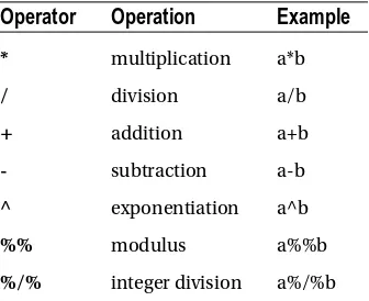
The arithmetic operators are the standard * for multiplication, / for division, + for addition, and - for subtraction. The exponentiation symbol is ^. The operator %% gives the modulus of the first argument with respect to the second argument. The operator
%/% performs integer division. Expressions can be grouped using parentheses, for example (a+b)/c. Table 3-2 lists the arithmetic operators.
Table 3-2. Arithmetic Operators
Operator
Operation
Example
* multiplication a*b
/ division a/b
+ addition a+b
- subtraction a-b
^ exponentiation a^b
%% modulus a%%b
For more information, the CRAN help pages for arithmetic operators can be found by entering ??“arithmetic operators” at the R prompt.
Matrix Operators and Functions
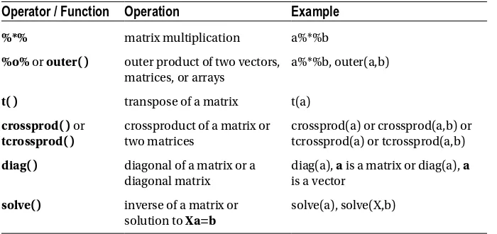
R provides operators and functions to manipulate matrices. A list of some matrix operators and functions can be found in Table 3-3.
Table 3-3. Matrix Operators and Functions
Operator / Function
Operation
Example
%*% matrix multiplication a%*%b
%o% or outer( ) outer product of two vectors, matrices, or arrays
a%*%b, outer(a,b)
t( ) transpose of a matrix t(a)
crossprod( ) or
tcrossprod( )
crossproduct of a matrix or two matrices
crossprod(a) or crossprod(a,b) or tcrossprod(a) or tcrossprod(a,b)
diag( ) diagonal of a matrix or a diagonal matrix
diag(a), a is a matrix or diag(a), a
is a vector
solve() inverse of a matrix or solution to Xa=b
solve(a), solve(X,b)
The matrix multiplication operator is %*%. R will return an error if the two matrices do not conform.
For two arrays (arrays include vectors and matrices), %o%, or outer(), gives the outer product of the arrays.
To transpose a matrix, use the function t(), for example, t(a).
To get the cross product of one matrix with another (or the original matrix), use either the function crossprod() or the function tcrossprod(). If a and b are conforming matrices, then
crossprod(a) = t(a)%*%a,
tcrossprod(a) = a%*%t(a),
crossprod(a,b) = t(a)%*%b,
17
To find the inverse of a nonsingular square matrix, use the function solve(), for example, solve(a). The function solve() also can solve the linear equation
Xa=b,
for a, where X is a nonsingular square matrix and b has the same number of rows as X. The syntax is solve(X,b).
To create a diagonal matrix or obtain the diagonal of a matrix, use the function diag(). If a is a vector, diag(a) will return a diagonal matrix with the diagonal equal to the a. For example:
> a = 1:2 > a [1] 1 2
> diag(a) [,1] [,2] [1,] 1 0 [2,] 0 2
If a is a matrix, diag(a) will return the diagonal elements of the matrix, even if the matrix is not square. For example:
> a = matrix(1:6,2,3)
> a
[,1] [,2] [,3] [1,] 1 3 5 [2,] 2 4 6
> diag(a) [1] 1 4
For more information, the CRAN help page for matrix multiplication can be found by entering ??“matrix multiplication” at the R prompt. For the five functions, entering
?name, where name is the name of the function, brings up the help page for the function.
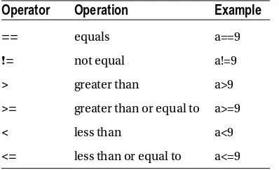
Relational Operators
Relational operators are used in logical tests. The six relational operators are == for equal to, != for not equal to, < for less than, <= for less than or equal to, > for greater than, and
Table 3-4. Logical Operators
Operator
Operation
Example
== equals a==9
!= not equal a!=9
> greater than a>9
>= greater than or equal to a>=9
< less than a<9
<= less than or equal to a<=9
Note that the equal to relational operator is ==, not =. A common mistake is to enter
= for == in a logical expression. R will return an error for =.
As with arithmetic operators, logical expressions can be grouped using parentheses. For example,
(( a>0 & b>0 ) & ( a<5 & b<5 ))
is a logical expression and can be assigned a name.
The CRAN help page for relational operators can be found by entering ??“relational operators” at the R prompt.
Subscripting Operators
Many objects in R have more than one element. Subscripting is used to access specific elements of an object. Vectors, matrices, arrays, lists, and slots can be subscripted. Single square brackets ([]), double square brackets ([[]]), dollar signs ($) and at symbols (@) are used for subscripting. None are used elsewhere.
Vectors
For vectors, using single square brackets is usually appropriate. Double square brackets can also be used, but they can only access a single element of the vector at a time. Within single square brackets, there may be a logical expression or a set of indices. For example:
a[ 3:7 ] or a[ a>3 ]
The first expression results in the third through seventh elements of a. The second expression results in those elements of a that are greater than three.
If indices are given a negative sign, those indices are not included For example,
a[ -2:-6 ]
19
An object can be subsetted in one set of square brackets and subsetted again in another set of square brackets. For example:
a[1:10][b>3],
where the length of a is greater than or equal to ten, and b is of length ten. The expression would return those elements of the first ten elements of a for which the corresponding element of b is greater than three. The subsetting can be continued with more sets of square brackets. Each set will operate on the result of all previous subsetting.
Matrices
For matrices, both kinds of square brackets are also used. For single square brackets, the selection instructions for the rows are separated from the selection instructions for the columns by a comma. Like the subsetting for vectors, for single square brackets, indices or a logical expression may be used to subset a matrix. To reference all rows of a matrix, put nothing to the left of the comma inside the brackets. To reference all columns of a matrix, put nothing to the right of the comma inside the brackets.
Double square brackets return just one value. If subsetted with a row and a column index separated by a comma, the value in the cell is returned. If just one index value is entered within double square brackets, R treats the matrix as a vector—going down rows—and returns the indexed element of the vector.
An example of matrix subscripting is
a[ a[,1]>3 , 1:4 ],
where a is a matrix with at least four columns. The expression would return those rows of the first four columns for which the elements of the first column are bigger than three. Notice that the a[,1] consists of one column and contains all of the rows.
A matrix can also be subsetted using a matrix with two columns. The two-column matrix would contain row and column indices and would pick out individual cells in the matrix based on the indices in each row. For example, if b is a matrix with [ 1 2 ] in the first row and [ 2 3 ] in the second row, then a[b] would return the two elements a[1,2] and a[2,3].
Arrays
Arrays are like matrices but can have more than two dimensions. Note that a matrix is an array with two dimensions and a vector is an array with one dimension. Subscripting arrays with more than two dimensions is just like subscripting matrices except that, for single square brackets, there are more commas in the brackets. An example is
a[ 1:3,,2:7 ],
Like matrices, arrays can be subsetted using a matrix that has the same number of columns as the number of dimensions of the array, the rows of which would consist of indices for individual cells of the array.
Lists
Lists are collections of R objects. The objects can be any type of object and do not have to be of the same type within a list. The objects are indexed in the list. To look at objects in a list, single square brackets are used. For example,
blist[ 1:5 ]
would return the first five objects in blist and would also be a list.
To access an object in a list, double square brackets or a dollar sign are required. For example,
blist[[2]]
would return the second object in the list blist and
blist$b1
would return the object in blist with name b1. Objects in a list can only be accessed one at a time.
If a list is created from objects that do not have names associated with the objects, names will be given to the objects when the list is created. Names can be changed at any time.
Data frames are a special kind of list. Data frames have the same number of elements for every object in the list and are defined as data.frames. Data frames can be subsetted like a matrix or like a list. If subsetted like a matrix, the resulting object will be a list. If subsetted like a list, the resulting object will be raw, complex, numeric, logical, or character depending on whether the list object is raw, complex, numeric, logical, or character. Individual cells in a data.frame can be accessed using indices in the double square brackets. For example,
adframe[[ 1,2 ]]
would return the element in the first row and second column of list adframe. Many functions return output in lists. Dollar sign subscripting is usually used to access the output, although square bracket indexing can be used. For example, for the linear model function lm(), entering
lm(y~x)$resid
or
21
will return the residuals from a simple linear regression of y on x, as will the two sets of statements
a=lm(y~x) a$resid
or
a=lm(y~x) a[[2]].
Other Types
Two other types of object can be subsetted—factors and slots. Objects that are factors are vectors and can be subsetted like vectors. Slots are a newer type of object and are subsetted using @. More information about subsetting both can be found by entering
??“Extract or Replace” at the R prompt.
Odds and Ends
Two object systems—S3 and S4—are used in R. Slots are part of S4. S3 and S4 are discussed in Chapter 4 and in the pdf at www.r-project.org/conferences/useR-2004/ Keynotes/Leisch.pdf.
Assignments can be done to subsets of an object. For example, let a be a matrix and let the user want to change those values in a that are greater than 100 to 100. Then the statement
a[ a>100 ] = 100
will do the replacement and leave the rest of the matrix intact.
The ? and ?? operators open the help pages. For known function names, ?name (or help(name)) will return the help page for the function, where name is the name of the function. To search for functions related to some techniques or methods, the operator, ?? is used. Entering ??“keywords” (or help.search(“keywords”)), where keywords consists of keywords about the technique or method, may give a list of functions in packages related to the topic. Sometimes the search comes up blank. Try again with different keywords.
The colon is used in four ways in R. Of interest here is just the use of a single colon to define a sequence and the double colon to refer to functions by package and name.
If a and b are two numbers, the expression a:b will give the sequence of integers between a rounded down to an integer and b rounded down to an integer. Note that the number a can be larger than the number b.
For more information on colons, enter ?“:” at the R prompt.
The operator ~ is used in model formulas to separate the left and right sides of a model. For more information, type ?“~” at the R prompt.
The symbol # is used for comments. When writing functions, anything found to the right of a # on a line of the code is ignored.
Kinds of Objects
Part II covers the different kinds of objects that are used in R in terms of their two important qualities: mode and class.
Chapter 4 lists the modes and describes the common ones. In addition to listing all of the modes current in R, the chapter describes the properties of the atomic modes—NULL, raw, logical, numeric, complex, and character—and of the nonatomic modes list, function, call, name, and expression.
Chapter 5 introduces the classes and gives the properties of several of them. The chapter includes a special section on vectors, which are not a class but, a very common kind of object. The classes associated with vectors are raw, logical,
integer, double, complex, character, some lists, and expressions. For most atomic objects, the mode and the class are the same. After describing vectors, we give properties of the classes for matrices, arrays, time series, factors, data frames, dates, and times and dates.
Modes of Objects
R objects exist within an object system. R has two object systems: S3 and S4. S4 is the newest version of R and contains a new way to approach R programming. S3 is the preceding version. Both versions run concurrently. S4 offers powerful new methods, but to use those methods a solid knowledge of S3 is necessary. This book focuses mainly on S3 methods, including S4 syntax where appropriate.
Overview of the Modes
Modes describe the type of information an object contains and are an S3-level classification. The mode of an object can be found by using the function mode(). The S4 level classification is by type and can be found using the function typeof(). Currently, R objects fall into one of the following modes: NULL, logical, numeric, complex, raw, character, list, expression,
name, function, pairlist, language, char, ..., environment, externalptr, weakref,
closure, bytecode, promise, and S4. Since R is constantly changing, the list of modes may change. With a few exceptions, the types and the modes are the same and most of the modes can be found under the list of types. The list of types can be found at the help page for typeof() and at http://svn.r-project.org/R/trunk/src/main/util.c, under the TypeTable. The instances for which mode() and typeof() give different results include the following: the function typeof() returns either integer or double where mode() returns numeric, typeof() returns either special or built-in where mode() returns function, and
typeof() returns symbol where mode() returns name. The help page for mode() gives the cross reference between modes and types.
Commonly Used Modes
Most users will never use half of the modes. The commonly used modes are NULL, logical,
numeric, complex, raw, character, list, function, call, name, expression, and S4. The mode NULL is the mode of an otherwise modeless empty object. Objects of mode logical
contain elements that can take on the values TRUE, FALSE, or NA, where NA represents a missing value. Objects of mode numeric can take on integer or real numeric values or
26
Objects of mode character are made up of character strings or NAs. The elements of character objects are quoted, except for NAs. Objects of mode list are lists of other objects, which can be of any mode. Objects of mode function are functions. Objects of mode name are a simplified name of an object based on the first element of the object, assuming the first element is not missing. Objects of mode call are functions and arguments. Objects of mode expression are collections of objects such as calls and names. Objects of mode S4 are those S4 objects that are complex (referring to the structure of the object, not to complex numbers).
The sources for the preceding information are the help pages for mode() and typeof().
Atomic, Recursive, and Language Modes
Modes come in three kinds: atomic, recursive, and language. The atomic modes are NULL,
logical, numeric, complex, raw, and character. Atomic refers to the elements of the objects being atomlike. For the atomic modes, all of the elements within the object are of the same atomic mode. Recursive modes are collections of objects and can contain objects of different modes. Two types of recursive modes are list and function. Most objects that are not atomic are recursive. The language modes are name, call, and
expression. More information about the kinds of modes can be found under the help pages for the functions that test for the kind of mode of an object: is.atomic(),
is.recursive(), and is.language().
Some Functions for Atomic Modes
Each of the atomic modes, except NULL, has three functions associated with the mode: the function named for the mode, name(); an as.name() function; and an is.name()
function, where name is the name of the mode. The name() function creates a vector of the length given by the argument or arguments, if the argument(s) are of the correct mode and permissible value(s).
The as.name() function attempts to coerce the argument of the function to the named mode. If the coercion is not possible, the as.name() function returns a vector of NAs or gives an error. Note that if the argument is a matrix or array, a vector of the elements of the matrix or array will be returned, where the conversion to a vector proceeds down each dimension of the matrix or array in turn (in the case of a matrix, going down the rows of the first column, then the second column, and so on).
The is.name() function tests whether the argument of the function is of the named mode and returns TRUE or FALSE, depending on whether the argument is or is not.
The NULL Mode
NULL is a reserved object in R and is also a mode. While there is no function NULL() in R,
The Logical Mode
The function logical() with no argument or with zero for an argument returns
logical(0), which is the logical empty set and has length zero. The function logical()
with an integer greater than zero as an argument returns a vector of FALSEs of length equal to the integer. If the argument is a single double precision element, the element is rounded down and a vector of FALSEs of the length equal to the resulting integer is created. If the argument is a numeric object other than a single number or if the argument is a logical object, the function returns FALSE. If the argument is of mode NULL,
character, complex, raw, or a nonatomic mode, then logical() gives an error. The function as.logical() coerces the argument of the function to logical, if possible, and returns a vector containing TRUEs, FALSEs, and/or NAs. If there is no argument or the argument is zero or NULL, as.logical() returns logical(0), a logical empty set of length zero. If the argument is of mode numeric, zeroes will be returned as
FALSEs and all other numbers will be returned as TRUEs.
If the argument is a complex object, the function returns FALSE for 0+0i and TRUE
for any other complex number. If the mode is raw, 00s will return FALSE and any other value will return TRUE. If the argument is of mode character, the function returns a vector of NAs of length equal to the length of the argument. If the argument contains NAs, for any of the modes except raw, NAs will be returned for the elements containing NAs. For the raw mode, there are no NAs since NAs are interpreted as 00s in the raw mode. For any other mode, as.logical() gives an error.
The function is.logical() returns TRUE if the argument is a logical object and
FALSE otherwise. The result of is.logical(logical(0)) is TRUE.
For more information about the logical mode, enter ?logical at the R prompt.
The Numeric Mode
For the mode numeric, things get a bit complicated. Originally in S, numeric objects could be integer, real, or double (for double precision). The real option is deprecated and should not be used. In S3, the integer and double options are both under mode
numeric. In S4, each has a separate type. The functions numeric(), is.numeric(), and
as.numeric() ae covered here. The functions integer(), as.integer(), is.integer(),
double(), as.double(), and is.double() behave similarly but are not covered here because they are at the S4 level.
The function numeric() takes a numeric object or NULL as an argument. If the argument equals zero or NULL or there is no argument, numeric() returns numeric(0), an empty object of mode numeric and length zero. If a numeric object of length greater than one or a logical object is the argument, only the first element is evaluated. For a logical
argument, TRUE is coerced to one and FALSE is coerced to zero, while for a numeric
argument, the first element is rounded down to an integer. The function then returns a vector on zeroes of length equal to the value of the first element. For arguments of modes other than numeric or logical, R returns an error.
28
the object. If the object is numeric, the values of the elements are returned as double precision numbers. If the object is complex, only the real parts are returned—as double precision numbers. If the object is of mode raw, as.numeric() converts the hexadecimal values to double precision. If the object is of mode character, the function returns NAs for the elements of the object. If the argument is not atomic, R gives an error. Elements with a value of NA are returned as NA.
The function is.numeric() tests an object to see if the object is a numeric object and works with objects of any mode. The value TRUE is returned if the object is numeric and
FALSE otherwise.
More information about mode numeric objects can be found by entering ?numeric
at the R prompt.
The Complex Mode
The complex mode is the mode of complex numbers. Complex numbers can be created using complex() or by simply typing in the numbers at the R prompt. For example:
> a = complex(real=1:5, imaginary=6:10) > a
[1] 1+ 6i 2+ 7i 3+ 8i 4+ 9i 5+10i
> a = 1:5 + 1i*6:10 > a
[1] 1+ 6i 2+ 7i 3+ 8i 4+ 9i 5+10i
Note that for complex numbers there is always a number with no operator in front of the i, which lets R know that the i is the imaginary root of minus one.
For the function complex(), an argument of zero or no argument returns complex(0), an empty set of mode complex and length zero. If the argument is a single positive number, complex() returns a vector of complex zeroes of the length of the number rounded down to an integer. If the argument consists of a numeric object with more than one element or if the argument is logical either with one element or more than one element, only the first element of the argument is used, where for logical objects FALSE is coerced to zero and TRUE to one.
The function complex() also take the arguments real and imaginary or modulus
and argument. The arguments real and imaginary or modulus and argument can be set equal to any numeric or logical objects. The objects do not have to be the same length and will cycle. The arguments real and imaginary are the real and imaginary parts of the numbers while the arguments modulus and argument are the polar coordinates of the numbers, with modulus equal to the lengths of the numbers and argument equal to the angles above the x axis of the numbers in radians.
Numbers of mode raw can be used for the real and imaginary arguments and will be changed to double precision, but they cannot be used for the modulus and argument
argument will be set to zero. For the modulus and argument pair, if modulus is omitted, the value for modulus will be set to one, and if argument is omitted, the value for
argument will be set to zero. Some examples of complex() include the following:
> complex(real=c(T,F), imaginary=1:5+0.5) [1] 1+1.5i 0+2.5i 1+3.5i 0+4.5i 1+5.5i
> complex(modulus=c(1,2), argument=pi/4) [1] 0.7071068+0.7071068i 1.4142136+1.4142136i
> as.raw(27:30) [1] 1b 1c 1d 1e
> complex(real=as.raw(27:30)) [1] 27+0i 28+0i 29+0i 30+0i
> complex(ima=as.raw(27:30)) [1] 0+27i 0+28i 0+29i 0+30i
> complex(mod=as.raw(27:30))
Error in rep_len(modulus, n) * exp((0+1i) * rep_len(argument, n)) : non-numeric argument to binary operator
> complex(mod=3:5) [1] 3+0i 4+0i 5+0i
> complex(arg=3:5*pi/180)
[1] 0.9986295+0.0523360i 0.9975641+0.0697565i 0.9961947+0.0871557i
The function as.complex( ) will try to coerce an object to mode complex. If the object can be coerced to numeric (the atomic modes) but is not complex, then the result is a complex object with the coerced argument as the real part and with zeros for the imaginary part, except for NAs, which are returned simply as NAs. For nonatomic modes,
as.complex() returns an error.
The function is.complex() tests whether the argument to the function is of mode
complex. The function returns TRUE if the argument is of the complex mode and
FALSE otherwise.
More information about the complex mode can be found by entering ?complex at the R prompt.
The Raw Mode
30
The function raw() returns a vector of 00s of length specified by the argument. If no argument or an argument of zero is given, raw() returns raw(0), an raw empty set with length zero. If a single number is entered as the argument, raw() returns a vector of length equal to the number rounded down to an integer. If any other kind of object is entered as the argument, raw() gives an error.
The function as.raw() attempts to coerce the argument of the function to raw. If no argument is given, as.raw() returns an error. If the argument is NULL, as.raw()
returns raw(0), the raw empty set. If the argument is zero, the function returns 00, the hexadecimal zero.
Objects of any of the atomic modes can be used as arguments for as.raw(). For logical mode objects, FALSEs are set to 00 and TRUEs are set to 01. For numeric mode objects, for values greater than or equal to zero and less than 256, the numbers are rounded down to an integer and converted to hexadecimal. Numbers outside the legal range are converted to 00. For objects of mode complex, the real portion is treated in the same way as numeric objects and the imaginary portion is discarded. For objects of mode character, all of the elements are converted to 00. Any element equal to NA
will also be set to 00. Using objects of modes other than atomic modes for the argument gives an error.
The function is.raw() tests if an object is of mode raw. The function returns TRUE if the object is of mode raw and FALSE otherwise. Any object can be used as an argument to is.raw().
More information about the mode raw can be found by entering ?raw at the R prompt.
The Character Mode
Character mode objects are made up of quoted strings. If an object is text, the text will be broken at each 500 characters to form a vector of strings. The three usual functions also apply to the character mode.
The function character() creates a vector of empty strings and only takes mode
numeric, one-element arguments. If the argument is greater than or equal to one, the argument is rounded down to an integer and the function returns a vector of “”s of length equal to the integer. If the argument is less than one and greater than or equal to zero, the character empty set of length zero, character(0), is returned. Other arguments return an error.
The function as.character() tries to convert the argument to strings. For the atomic modes, the conversion is literal, but the elements are returned within quotes. For double precision numbers up to 15 significant digits are used. Unlike the other atomic modes—except NULL—the function as.character() also returns results for some of the recursive modes.
Objects of mode list are described under the next section. In this section, lists are collections of objects that can be of any mode. The function lm() used in the example below fits a linear regression model, with the value to the left of the tilde being the dependent variable and the value to the right the independent variable. The output from
With an object of mode list as an argument, as.character() may return some strange things depending on the list. The function may return something different from what is returned if the argument is entered at the R prompt. Examples follow:
> a.list [[1]]
a1 a2 a3 a4 [1,] 1 6 11 16 [2,] 2 7 12 17 [3,] 3 8 13 18 [4,] 4 9 14 19 [5,] 5 10 15 20
[[2]]
[1] 1 2 3 4 5 6 7 8 9 10
[[3]]
[1] "glh" "abc"
> as.character(a.list)
[1] "1:20" "1:10" "c(\"glh\", \"abc\")"
> a.lm
Call:
lm(formula = y ~ x)
Coefficients:
(Intercept) x 1 1
> as.character(a.lm)
[1] "c(0.999999999999999, 1)" [2] "c(0, 0, 0)"
[3] "c(-5.19615242270663, -1.41421356237309, 0)" [4] "2"
[5] "c(2, 3, 4)" [6] "0:1"
[7] "list(qr = c(-1.73205080756888, 0.577350269189626, 0.577350269189626, -3.46410161513776, -1.41421356237309, 0.965925826289068), qraux =
c(1.57735026918963, 1.25881904510252), pivot = 1:2, tol = 1e-07, rank = 2)" [8] "1"
[9] "list()"
[10] "lm(formula = y ~ x)" [11] "y ~ x"
32
Play around with different kinds of lists to see how as.character() performs. Objects of modes name, call, and expression can also be coerced to character. Objects of modes function and S4 cannot.
The function is.character( ) tests to see if the argument to the function is of mode character and returns TRUE if so and FALSE otherwise. Any object can be used as an argument.
For more information about the character mode, enter ?character at the R prompt.
The Common Recursive and Language Modes
The recursive and language modes covered in this book are list, function, call,
expression, and name. The modes list, function, call, and expression are all recursive modes. The modes call and expression are also language modes. The mode name is a language mode but not a recursive mode.
The List Mode
Lists are collections of objects, which may be of any mode and which do not have to be of the same mode within the list. The list mode has the same three functions as the atomic modes; however, there are a few more. Creating an empty list differs from the atomic modes. To create a list of a given number of objects where the objects are NULLs, use
vector("list", n),
where n is the number of objects to be in the list. The variable, n, must be numeric, is rounded down to an integer, and can only contain one element.
The function unlist() removes the list property for some lists and, for those lists, returns a vector of the elements of the objects in the list.
The function alist() creates a list where the values of variables in the list do not have to be specified. The function alist() is most often used in evaluating functions, where some variables can be prespecified and others are assigned at each running of the function.
The function list() creates a list out of the arguments to the function. Within the parentheses, the arguments are separated by commas. The arguments can be any kind of object.
The function as.list() attempts to coerce the argument to mode list. If more than one argument is supplied, only the first argument is coerced. The other arguments are ignored.
The function is.list() tests if the argument is a list (or a pairwise list, which is not covered here). If the object is of mode list, TRUE is returned. Otherwise, FALSE
is returned.
The Function Mode
Functions in R are of mode function. Of the functions listed for atomic modes, only
is.function() and function() exist for the mode function. The function is.function()
returns TRUE if the argument is a function and FALSE otherwise. The function
function() creates functions, but the structure of functions is different from the atomic modes and the list mode, and the help page for function() is different from the help page for is.function(). We will cover the creation of functions in Chapter 7.
Another mode for functions is closure. The mode closure is for functions that are not primitive—that is, are written in R code. Note that functions of mode closure are also of mode function. The function is.primitive() exists to test if a function is primitive, but a function is.closure() does not exist.
More information about the function mode can be found by entering ?is.function
at the R prompt, which will bring up the help page for is.function().
The Call Mode
Objects of the call mode are unevaluated functions with arguments, if the function takes arguments. The same three functions that exist for the atomic modes exist for the call
mode: call(), as.call(), and is.call().
The function call() creates an object of mode call. The first argument of call() is the name of the function in quotes. The rest of the arguments to call are the arguments to the function. Some examples include the following:
> a.call = call("lm", y~x) > a.call
lm(y ~ x)
> b.call = call("ls") > b.call
ls()
> c.call = call("ls", pattern="abc") > c.call
ls(pattern = "abc")
Note that an object of mode call can be evaluated using the function eval(). If all of the variables in the call exist in the workspace, eval() will evaluate the function; otherwise eval() will give an error. For example:
34
Call:lm(formula = y ~ x)
Coefficients:
(Intercept) x 1 1
> a.call = call("lm", z~x) >
> z
Error: object 'z' not found >
> eval(a.call)
Error in eval(expr, envir, enclos) : object 'z' not found
The function as.call() tries to coerce the argument to an object of mode call. If the argument is a list, then the conversion takes place; otherwise an error is returned. However, if the list does not consist of the name of a function followed by the arguments of that function, the object cannot be evaluated.
The function is.call() tests the argument and returns TRUE if the argument is of mode call and FALSE otherwise.
Further information about the mode call can be found by entering ?call at the R prompt.
The Name Mode
The mode name refers to objects that are names created for and from other objects. Only the functions as.name() and is.name() exist for the name mode. Names can be up to 10,000 bytes long.
The function as.name() takes arguments that can be logical, numeric, complex,
raw, character, or name. Arguments of other modes give an error. The function uses the first element of the object to assign the name. For example:
> mat one two row1 1 6 row2 2 7
> as.name(mat) `1`.
The function is.name() tests if the argument is of mode name and returns TRUE if so and FALSE otherwise.
The Expression Mode
The expression mode is like the list mode, but mainly for objects of modes like class
or name. Objects of mode expression can be subsetted like lists and are not evaluated when created. The expression mode uses the three functions that the atomic modes use:
expression(), as.expression(), and is.expression().
The function expression() creates a listing of the objects entered into the function. The objects are separated by commas and can be of any mode. The function eval() can be used to evaluate the expression. Only the last object in an expression is evaluated under eval(). If the last argument is made up of primitive functions, eval() will return the result, while if the function or expression is not primitive, eval() will return the expression. A second eval() is then necessary to evaluate the function or expression. Examples follow:
> a.exp = expression(sin(1:5/180*pi)) > a.exp
expression(sin(1:5/180 * pi)) > eval(a.exp)
[1] 0.01745241 0.03489950 0.05233596 0.06975647 0.08715574
> a.exp = expression(sin(1:5/180*pi),a.call) > a.exp
expression(sin(1:5/180 * pi), a.call) > eval(a.exp)
lm(y ~ x)
> eval(eval(a.exp))
Call:
lm(formula = y ~ x)
Coefficients:
(Intercept) x 1 1
> a.exp = expression(a.call,sin(1:5/180*pi)) > eval(a.exp)
[1] 0.01745241 0.03489950 0.05233596 0.06975647 0.08715574
An object of name mode will give an error if placed as the last argument in an expression that is being evaluated.
The function as.expression() attempts to coerce the argument to mode
expression. The modes NULL, call, name, and pairlist are coerced to a single element expression. Atomic modes other than NULL are coerced elementwise. Lists are coerced with no changes except the mode. Other modes of objects will give an error if coercion is atte