Full Terms & Conditions of access and use can be found at
http://www.tandfonline.com/action/journalInformation?journalCode=ubes20
Download by: [Universitas Maritim Raja Ali Haji], [UNIVERSITAS MARITIM RAJA ALI HAJI
TANJUNGPINANG, KEPULAUAN RIAU] Date: 11 January 2016, At: 21:00
Journal of Business & Economic Statistics
ISSN: 0735-0015 (Print) 1537-2707 (Online) Journal homepage: http://www.tandfonline.com/loi/ubes20
Asymptotic Theory for the QMLE in
GARCH-X Models With Stationary and Nonstationary
Covariates
Heejoon Han & Dennis Kristensen
To cite this article: Heejoon Han & Dennis Kristensen (2014) Asymptotic Theory for the QMLE in GARCH-X Models With Stationary and Nonstationary Covariates, Journal of Business & Economic Statistics, 32:3, 416-429, DOI: 10.1080/07350015.2014.897954
To link to this article: http://dx.doi.org/10.1080/07350015.2014.897954
View supplementary material
Accepted author version posted online: 10 Mar 2014.
Submit your article to this journal
Article views: 206
View related articles
View Crossmark data
Supplementary materials for this article are available online. Please go tohttp://tandfonline.com/r/JBES
Asymptotic Theory for the QMLE in GARCH-X
Models With Stationary and Nonstationary
Covariates
Heejoon H
ANDepartment of Economics, Kyung Hee University, Seoul 130-701, Republic of Korea ([email protected])
Dennis K
RISTENSENDepartment of Economics, University College London, London WC1E 6BT, United Kingdom; Center for Research in Econometric Analysis of Time Series (CREATES), University of Aarhus, Aarhus, Denmark; Institute for Fiscal Studies (IFS), London WC1E 7AE, United Kingdom ([email protected])
This article investigates the asymptotic properties of the Gaussian quasi-maximum-likelihood estimators (QMLE’s) of the GARCH model augmented by including an additional explanatory variable—the so-called GARCH-X model. The additional covariate is allowed to exhibit any degree of persistence as captured by its long-memory parameterdx; in particular, we allow for both stationary and nonstationary covariates. We
show that the QMLE’s of the parameters entering the volatility equation are consistent and mixed-normally distributed in large samples. The convergence rates and limiting distributions of the QMLE’s depend on whether the regressor is stationary or not. However, standard inferential tools for the parameters are robust to the level of persistence of the regressor witht-statistics following standard Normal distributions in large sample irrespective of whether the regressor is stationary or not. Supplementary materials for this article are available online.
KEY WORDS: Asymptotic properties; Persistent covariate; Quasi-maximum likelihood; Robust infer-ence.
1. INTRODUCTION
To better model and forecast the volatility of economic and financial time series, empirical researchers and practitioners of-ten include exogenous regressors in the specification of volatility dynamics. One particularly popular model within this setting is the so-called GARCH-X model where the basic GARCH speci-fication of Bollerslev (1986) is augmented by adding exogenous regressors to the volatility equation:
yt =σt(ϑ)εt, (1)
whereεtis the error process whileσt2(ϑ) is the volatility process
given by
σt2(ϑ)=ω+αyt2−1+βσt2−1+π xt2−1, (2) for some observed covariatext which is squared to ensure that
σ2
t(ϑ)>0, and whereϑ =(ω, θ′)′,θ=(α, β, π)′, is the
vec-tor of parameters. The inclusion of the additional regressorxt
often helps explaining the volatilities of stock return series, exchange rate returns series or interest rate series and tend to lead to better in-sample fit and out-of-sample forecasting performance. Choices of covariates found in empirical studies using the GARCH-X model span a wide range of various eco-nomic or financial indicators. Examples include interest rate levels (Glosten et al.1993; Brenner, Harjes, and Kroner1996; Gray 1996), bid-ask spreads (Bollerslev and Melvin 1994), interest rate spreads (Dominguez 1998; Hagiwara and Herce 1999), forward-spot spreads (Hodrick1989), futures open in-terest (Girma and Mougoue2002), information flow (Gallo and Pacini2000), and trading volumes (Lamoureux and Lastrapes 1990; Marsh and Wagner 2005; Fleming, Kirby, and Ostdiek
2008). More recently, various realized volatility measures con-structed from high-frequency data have been adopted covari-ates in the GARCH-type models with the rapid development seen in the field of realized volatility; see Barndorff-Nielsen and Shephard (2007), Engle (2002), Engle and Gallo (2006), Hansen, Huang, and Shek (2012), Hwang and Satchell (2005), and Shephard and Sheppard (2010).
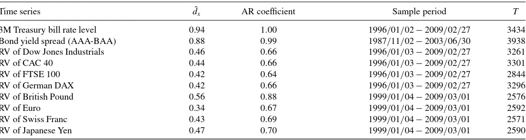
While the GARCH-X model and its associated quasi-maximum likelihood estimator (QMLE) have found widespread empirical use, the theoretical properties of the estimator are not fully understood. In particular, given the wide range of differ-ent choices of covariates, it is of interest to analyze how the persistence of the chosen covariate influences the QMLE. As shown inTable 1, the degree of persistence varies a lot across some popular covariates used in GARCH-X specifications. The table reports log-periodogram estimates of memory parameter,
dx, and estimates of the first-order autocorrelation,ρ1, for some time series used as covariates in the literature. For example, interest rate levels and bond yield spreads are highly persistent with estimates ofdx being mostly larger than 0.8 andρ1 esti-mates close to unity, thereby suggesting unit root type behavior. Meanwhile, realized volatility measures (realized variance) of various stock index and exchange rate return series are less per-sistent with estimates ofdxranging between 0.3 and 0.6 while
© 2014American Statistical Association Journal of Business & Economic Statistics July 2014, Vol. 32, No. 3 DOI:10.1080/07350015.2014.897954 Color versions of one or more of the figures in the article can be found online atwww.tandfonline.com/r/jbes. 416
Table 1. Estimates of memory parameterdxand AR(1) coefficient for various time series
Time series dˆx AR coefficient Sample period T
3M Treasury bill rate level 0.94 1.00 1996/01/02−2009/02/27 3434 Bond yield spread (AAA-BAA) 0.88 0.99 1987/11/02−2003/06/30 3938 RV of Dow Jones Industrials 0.46 0.66 1996/01/03−2009/02/27 3261 RV of CAC 40 0.44 0.66 1996/01/03−2009/02/27 3301 RV of FTSE 100 0.42 0.64 1996/01/03−2009/02/27 2844 RV of German DAX 0.42 0.66 1996/01/03−2009/02/27 3296 RV of British Pound 0.56 0.88 1999/01/04−2009/03/01 2576 RV of Euro 0.34 0.67 1999/01/04−2009/03/01 2592 RV of Swiss Franc 0.43 0.69 1999/01/04−2009/03/01 2571 RV of Japanese Yen 0.47 0.70 1999/01/04−2009/03/01 2590
NOTE: ˆdxis the log-periodogram estimate of the memory parameterdxandTis the number of observations. RV represents the realized variance of return series. All realized variance
series are from “Oxford-Man Institute’s realized library,” produced by Heber et al. (2009). (Seehttp://realized.oxford-man.ox.ac.uk/). All time series are at the daily frequency.
the estimates ofρ1 are relatively small and taking values be-tween 0.64 and 0.88; formal unit root tests clearly reject unit root hypotheses for these time series. A natural concern would be that different degrees of persistence of the chosen covariates would lead to different behavior of the QMLE and associated inferential tools.
We provide a unified asymptotic theory for the QMLE of the parameters allowing for both stationary and nonstationary regressors. In the stationary case, we do not impose any fur-ther restrictions on the dynamics ofxt. In the case of
nonsta-tionary regressors, on the other hand, we specifically model
xt as an I(dx) process with 1/2< dx<3/2. This allows for
a wide range of persistence as captured by the long-memory parameterdx, including unit root processes (dx=1) but also
processes with either weaker (dx<1) or stronger dependence
(dx >1).
Our main results show that to a large extent applied re-searchers can employ the same techniques when drawing in-ference regarding model parameters regardless of the degree of persistence of the regressors. We first show that QMLE consis-tently estimatesϑ0 whetherxt is stationary or not, but that its
convergence rates and limiting distribution changes whenxtis
nonstationary. In particular, its distribution is mixed-normal in the nonstationary case. At the same time, we also demonstrate that the large sample distributions of t-statistics are invariant to the degree of persistence and always followN(0,1) distri-butions. This last limit result is because in the computation of
t-statistics, the QMLE’s are normalized by estimators of the square root of its quadratic variation. In the stationary case, the estimated quadratic variation of the QMLE’s converge toward a constant as is standard. On the other hand, in the nonstationary case, the limiting quadratic variation is random which leads to the distribution of the QMLE’s to be mixed-normal. This self-normalization of the QMLE’s when computingt-statistics re-moves any non-Gaussian component of the limiting distribution of the QMLE’s and so the statistics converge towardN(0,1) distributions even in the nonstationary case. As consequence, standard inference tools are applicable whether the regressors are stationary or not, and so researchers do not have to conduct any preliminary analysis of a given covariate before carrying out inference in GARCH-X models. A simulation study con-firms our theoretical findings, with the distribution of standard
t-statistics showing little sensitivity to the degree of persistence of the included covariate.
Our theoretical results have important antecedents in the lit-erature. Our theoretical results for the nonstationary case rely on some of the results developed in Han (2014) and Han and Park (2013) who analyzed the time series properties of GARCH-X models with long-memory regressors. Kristensen and Rahbek (2005) provided theoretical results for the QMLE in the linear ARCH-X models in the case of stationary regressors. We extend their theoretical results to allow for lagged values of the volatil-ity in the specification and nonstationary regressors. Jensen and Rahbek (2004) and Franq and Zako¨ıan (2012) analyzed the QMLE in the pure GARCH model (i.e., no covariates included,
π =0) and showed that the QMLE of (α, β) remained con-sistent and√n-asymptotically normally distributed even when
σt2(ϑ) was explosive. On the other hand, they found thatωis not identified when the volatility process is nonstationary. Our results for the QMLE of θ are similar: It remains consistent and√n-asymptotically normally distributed independently of whetherx2
t, and therebyσ
2
t(ϑ), is explosive or not. However,
in contrast to the pure GARCH model, it is possible to iden-tify and consistently estimateωin the GARCH-X model even whenxtis nonstationary. But the QMLE of ofωconverges at a
slower rate in this case. The contrasting results regardingωare because the dynamics of a nonstationary pure GARCH process are very different from those of a GARCH-X process with non-stationarity being induced through an exogenous long-memory process.
Finally, Han and Park (2012), henceforth HP2012, estab-lished the asymptotic theory of the QMLE for a GARCH-X model where a nonlinear transformation of a unit root process was included as exogenous regressor. Our work complements HP2012 in that we allow for a wider range of dependence in the regressor, but on the other hand do not consider general non-linear transformations of the variable. In the special case with
dx =1, our results for the estimation ofθcoincide with those of
HP2012 with their transformation chosen as the quadratic func-tion. At a technical level, we provide a more detailed analysis of the QMLE compared to HP2012. While HP2012 conjectured thatωwas not identified and so kept the parameter fixed at its true value in their analysis, we here show that in fact ω can be consistently estimated from data and derive the large-sample
distribution of its QMLE. This last result is derived by extend-ing some novel limit results for nonstationary regression models developed in Wang and Phillips (2009a,b).
The rest of the article is organized as follows. Section2 intro-duces the model and the QMLE. Section3derives the asymp-totic theory of the QMLE and their correspondingt-statistics for the stationary and nonstationary case. The results of a simula-tion study is presented in Secsimula-tion4. Section5concludes. Proofs of theorems have been relegated to Appendix A, while proofs of lemmas can be found in the online supplemental material. Before we proceed, a word on notation: Standard terminologies and notations employed in probability and measure theory are used throughout the article. Notations for various convergences such as→a.s.,→p, and→d frequently appear, where all limits
are taken asn→ ∞except where otherwise indicated. 2. MODEL AND ESTIMATOR
The GARCH-X model is given by Equations (1)–(2), where the parameters are collected in ϑ=(ω, θ) where θ=
(α, β, π)∈⊆R3andω∈W⊆[0,∞). The chosen decom-position of the full parameter vector into θ and the inter-cept ω is due to the special role played by the latter in the nonstationary case. The true data-generating parameter is de-noted ϑ0=(ω0, θ0′)′, whereθ0=(α0, β0, π0)′ and the associ-ated volatility processσ2
t =σ
2
t(ϑ0). We will throughout assume thatE[log(α0εt2+β0)]<0 so that nonstationarity can only be induced byxt. In particular, ifxtis stationary thenσt2andytare
stationary; see Section3.1for details. In the stationary case, we impose no further restrictions on its time series dynamics. On the other hand, in the nonstationary case, we restrictxt to be a
long-memory process of the form
xt=xt−1+ξt, (3)
where, for a sequence{vt}which is iid (0, σv2),
(1−L)dξt =vt, −1/2< d <1/2. (4)
Hence, xt is anI(dx) process with dx =d+1∈(1/2,3/2).
Note that {εt}and {vt} are allowed to be dependent. Hence,
the model can accommodate leverage effects catered for by the GJR-GARCH model if{εt}and{vt}are negatively correlated.
See Han (2014) for more details on the model and its time series properties.
Dittmann and Granger (2002) analyzed the properties ofx2
t
givenxt is fractionally integrated and showed that whenxtis a
Gaussian fractionally integrated process of orderdx, thenxt2is
asymptotically also a long-memory process of orderdx2=dx.
Hence, for 1/2< dx <3/2,the covariatext2 is nonstationary
long memory, including the case of unit root-type behavior. Considering that the range of memory parameter for real data used as covariates in the literature seldom exceeds unity, the range ofdx we consider is wide enough to cover all covariates
used in the empirical literature.
Whetherxtis stationary or not, we will require it to be
exoge-neous in the sense thatE[εt|xt−1]=0 andE[ε2t|xt−1]=1. This restricts the choices ofxt; for example, in most situations, the
exogeneity assumption will be violated ifyt is a stock return,
say,r1,t andxt−1=r2,t is another return series since these will
in general be contemporaneously correlated. This in turn will
generate simultaneity biases in the estimation of the GARCH-X model similar to OLS in simultaneous equations models. If in-steadxt−1=r2,t−1, the GARCH-X model can be thought of as a restricted version of a bivariate GARCH model where lags of
r1,tdo not affect the volatility ofr2,t and only the first lag ofr2,t
affects the volatility ofr1,t. This restriction may in some cases
be implausible. On the other hand, GARCH-X models is a lot simpler to estimate compared to a bivariate GARCH model. The former only contains four parameters while a bivariate BEKK-GARCH(1,1) contains 12 parameters.
Our model is related to the one considered in HP2012 given byσ2
t (ϑ)=αyt2−1+βσ 2
t−1(ϑ)+f(xt−1, γ), wherext is
inte-grated or near-inteinte-grated, andf(xt−1, γ) is a positive, asymp-totically homogeneous function as introduced by Park and Phillips (1999). (Note a notational difference in HP2012: In-stead off(xt−1, γ), HP2012 usedf(xt, γ) wherext is adapted
toFt−1.) If we let dx =1 in our model,xt is integrated and
our model belongs to the model considered by HP2012 with
f(xt−1, γ)=ω+π xt2−1. While their model allows for more general nonlinear transformations ofxt, our analysis includes
more general dependence structure ofxt. It is either
stationar-ity or it is fractionally integrated process with 1/2< dx <3/2.
As shown in Table 1, these are empirically relevant types of dynamic behavior.
Let (yt, xt−1) for t=0, . . . , n, be n+1≥2 observations from (1)–(2). We then consider estimation ofϑ0using the Gaus-sian log-likelihood withεt ∼iidN(0,1):
Ln(ϑ)= n
t=1
ℓt(ϑ), ℓt(ϑ)= −logσt2(ϑ)−
yt2 σ2
t (ϑ)
,
whereσt2(ϑ) is given in Equation (2). The volatility process is assumed to be initialized at some fixed parameter-independent value ¯σ02>0, σ02(ϑ)=σ¯02. We will not restrictεt to be
nor-mally distributed and hence Ln(ϑ) is a quasi-log-likelihood.
The QMLE ofϑ0is then defined as:
ˆ
ϑ=( ˆω,θˆ)=arg max
(ω,θ)∈W×Ln(ω, θ). (5)
3. ASYMPTOTIC THEORY
The main arguments used to establish the asymptotic distri-bution of the QMLE are identical for the two cases—stationary or nonstationary regressors. The technical tools used to establish the main arguments differ in the two cases though, and so we provide separate proofs for them. But first, we outline the proof strategy for consistency and asymptotic normality of the QMLE to emphasise similarities and differences in the analysis of the two different cases.
To present the arguments in a streamlined fashion, it proves useful to redefine ℓt(ϑ) as a normalized version of the
log-likelihood function by subtracting the log-log-likelihood evaluated atϑ0,
ℓt(ϑ) :=
−logσt2(ϑ)− y 2
t
σt2(ϑ)
−
−logσt2− y 2
t
σt2
= −log (rt(ϑ))−
1
rt(ϑ)−
1
ε2t,
whereσt2denotes the true data-generating volatility process,
σt2 =ω0+α0yt2−1+β0σt2−1+π0xt2−1, (6) andrt(ϑ) is a variance-ratio process defined as
rt(ϑ) :=
σ2
t (ϑ)
σt2
. (7)
This normalization does not affect the QMLE since−logσ2
t −
y2
t/σt2 is parameter-independent. Note that the processrt(ϑ)
is in general not stationary sinceσ2
t (ϑ) has been initialized at
some fixed value andxtmay be nonstationary. For consistency,
the main argument involves showing that the normalized version of the log-likelihood satisfies
sup
ϑ∈W×
1
nLn(ϑ)−L ∗
n(ϑ) → P
0, (8)
whereL∗
n(ϑ) is given by
L∗n(ϑ)=
n
t=1 ℓ∗t (ϑ),
ℓ∗t (ϑ)= −log(rt∗(ϑ))−
1
r∗
t (ϑ)−
1
ε2t, (9)
and r∗
t (ϑ) is a stationary sequence which is asymptotically
equivalent tort(ϑ). We can now appeal to a uniform Law of
Large Numbers (LLN) for stationary and ergodic sequences to obtain thatL∗
n(ϑ)/n→p L∗(ϑ) :=E[ℓ∗t(ϑ)] uniformly inϑ.
The precise definition ofrt∗(ϑ), and therebyL∗(ϑ), depends on whetherxtis stationary or not. In particular, in the stationary case
ϑ0=arg maxϑL∗(ϑ) is uniquely identified and so ˆϑ→p ϑ0 globally, while in the nonstationary caseL∗(ϑ)=L∗(θ) is con-stant w.r.t.ωand so we can only conclude that ˆθ→p θ0. This would seem to indicate that in the nonstationary case ˆωis incon-sistent which would be similar to the explosive pure GARCH model as analyzed by Jensen and Rahbek (2004) and Franq and Zako¨ıan (2012). However, in our case, this conclusion is not correct and is an artifact of normalizingLn(ϑ) by 1/n. By
ana-lyzing the local behavior ofLn(ϑ) in a shrinking neighborhood
ofϑ0, we find that in the nonstationary case ˆωremains consistent but converges at a slower rate compared to ˆθ.
To derive the asymptotic distribution of ˆϑ, we proceed to ana-lyze the score and hessian of the quasi-log-likelihood. We denote the score vector by Sn(ϑ)=(Sn,ω(ϑ), Sn,θ(ϑ)′)′∈R4, where
Sn,ω(ϑ)=∂Ln(ϑ)/(∂ω)∈R and Sn,θ(ϑ)=∂Ln(ϑ)/(∂θ)∈
R3and the Hessian matrix by
Hn(ϑ)=
Hn,ωω(ϑ) Hn,ωθ(ϑ)
Hn,θ ω(ϑ) Hn,θ θ(ϑ)
∈R4×4, (10) whereHn,θ ω(ϑ)=∂2Ln(ϑ)/(∂θ ∂ω)∈R3and the other
com-ponents are defined similarly. A standard first-order Taylor expansion of the score vector yields 0=Sn( ˆϑ)=Sn(ϑ0)+ Hn( ¯ϑ)( ˆϑ−ϑ0), where ¯ϑ lies on the line segment connecting
ˆ
ϑandϑ0. Assuming thatϑ0lies in the interior of the parameter space, ˆϑmust be an interior solution with probability approach-ing one (w.p.a.1). That is,Sn( ˆϑ)=0 w.p.a.1. What remains is
to derive the limiting distribution ofSn(ϑ0) andHn( ¯ϑ).
In the stationary case, we can appeal to LLN and central limit theorem (CLT) for stationary and ergodic sequences to show
that
Sn(ϑ0)/
√
n→d N(0, st), −Hn( ¯ϑ)/n→pHst>0, (11)
where st
∈R4×4 are Hst
∈R4×4 are constant. This implies that
√
n( ˆϑ−ϑ0)→d N(0, st), st=(Hst)−1st(Hst)−1. (12)
In the nonstationary case, the score and Hessian, and thereby the QMLEs, have different asymptotic behavior. First of all, ˆω
and ˆθconverge at different rates which we collect in the matrix
Vn,
Vn:=
n1/4−d/2 O 1×3 O3×1 n1/2I3
∈R4×4, (13)
whereOk×m∈Rk×mdenotes the matrix of zeros andIk∈Rk×k
denotes the identity matrix. We then show that
Vn−1Sn(ϑ0)→d MN(0, nst),
−Vn−1Hn( ¯ϑ)Vn−1→d Hnst>0, (14)
where MN(0, nst) denotes a mixed-normal distribution with (random) covariance matrix nst
∈R4×4, and Hnst
∈R4×4 is also random. The proof of Equation (14) employs generalized versions of limit results for fractionally integrated processes developed in Wang and Phillips (2009a) that we have collected in Theorem 6. Having established (14), it follows by standard arguments that
Vn( ˆϑ−ϑ0)→d MN(0, nst), nst =(Hnst)−1nst(Hnst)−1.
(15)
In particular, ˆθis√n-asymptotically normally distributed while ˆ
ωconverges with a slower rate ofn1/4−d/2and follows a mixed-normal distribution. Importantly, in comparison to pure explo-sive GARCH models, whereω0 is not identified, we can still conduct inference aboutω0when the explosiveness is induced by a long-memory regressor.
In conclusion, the asymptotic distribution of ˆϑ depends on whetherxt is stationary or not. Fortunately, the distribution is
in both cases mixed-normal and so standard test statistics prove to be robust to the degree of persistence of xt. In particular,
we show that standardt-statistics followN(0,1) distributions irrespective of the regressor’s level of persistence. The reason for this result is that in the computation of thet-statistics, we premultiply the QMLEs with an estimator of its large-sample covariance matrix. This normalization takes out the random covariance matrix,nst, that appears in the limiting distribution in the nonstationary case.
Since the assumptions and techniques used to establish the above results differ depending on whether xt is stationary or
not, we consider the two cases in turn. The following section covers the stationary case, while the subsequent one focuses on the nonstationary case. Based on these results, the asymptotic properties of thet-statistics are analyzed in Section3.3.
3.1 QMLE in Stationary Case
We first show that the QMLE is globally consistent under the following conditions withFtdenoting the natural filtration:
Assumption 1.
(i) {(εt, xt)}is stationary and ergodic with E[εt|Ft−1]=0 andE[ε2
t|Ft−1]=1.
(ii) E[log(α0εt2+β0)]<0 and E[x 2q
t ]<∞ for some 0<
q <∞.
(iii) = {ϑ :ω≤ω≤ω,¯ 0≤α≤α¯, 0≤β ≤β¯, 0≤π ≤
¯
π}, where 0< ω≤ω <¯ ∞, ¯α <∞, ¯β <1 and ¯π <∞. The true valueϑ0∈with (α0, π0)=(0,0).
(iv) For any (a, b)=(0,0):aε2
t +bxt2|Ft−1has a nondegen-erate distribution.
Assumption 1(i) is a generalization of the conditions found in Escanciano (2009) who derived the asymptotic properties of QMLE for pure GARCH processes (i.e., no exogenous co-variates are included) with martingale difference errors. The assumption is weaker than the iid assumption imposed in Kris-tensen and Rahbek (2005). The moment conditions in As-sumption 1(ii) implies that a stationary solution to Equations (1)–(2) at the true parameter valueϑ0 exists and has a finite polynomial moment; see Lemma 1. We here allow for inte-grated GARCH processes (α+β =1), and impose very weak moment restrictions on the regressor. We do, however, rule out explosive volatility when xt is stationary; we expect that
the arguments of Jensen and Rahbek (2004) can be extended to GARCH-X models with E[log(α0εt2−1+β0)]>0, thereby showing that ˆθis consistent while ˆωis inconsistent. The com-pactness condition in Assumption 1(iii) should be possible to weaken by following the arguments of Kristensen and Rahbek (2005); this will lead to more complicated proofs though and so we maintain the compactness assumption here for simplic-ity. The requirement that (α0, π0)=(0,0) is needed to ensure identification of β0 since in the case where (α0, π0)=(0,0), σ2
t =σt2(ϑ0)→a.s.ω0/(1−β0) and so we would not be able to jointly identifyω0 andβ0. The nondegeneracy condition in Assumption 1(iv) is also needed for identification. It rules out (dynamic) collinearity betweenyt2−1 andx2
t. It is similar to the
no-collinearity restriction imposed in Kristensen and Rahbek (2005).
To derive the asymptotic properties of ˆϑ, we establish some preliminary results. The first lemma states that a stationary so-lution to the model at the true parameter values exists:
Lemma 1 (Under Assumption 1). There exists a
station-ary and ergodic solution to Equations (1)–(2) atϑ0 satisfying
E[σt2s]<∞andE[yt2s]<∞for some 0< s <1.
We will in the following work under the implicit assumption that we have observed the stationary solution. Next, we show that for any value ofϑin the parameter space, the volatility-ratio processrt(ϑ) is well-approximated by a stationary version.
Lemma 2 (Under Assumption 1). Withs >0 given in Lemma
1, there exists someKs <∞such that
E
sup
ϑ∈W×
rt(ϑ)−rt∗(ϑ)
s
≤Ksβst,
where
rt∗(ϑ) := σ
2 0,t(ϑ)
σ2
t
,
σ02,t(ϑ) :=
∞
i=1 βi−1
ω+αyt2−i+π xt2−i
. (16)
The process σ2
0,t(ϑ) is stationary and ergodic with
E[supϑ∈W×σ
2s
0,t(ϑ)]<∞.
Note that, in particular,σt2=σ02,t(ϑ0). This in turn implies that Equation (8) holds with rt∗(ϑ) defined in the previous lemma. With these results in hand, we are now ready to show the first main result of this section.
Theorem 3. Under Assumption 1, the QMLE ˆϑis consistent.
Having shown that the QMLE is consistent, we proceed to verify Equation (11) under the following additional assumption:
Assumption 2.
(i) κ4=E[(εt2−1)2|Ft−1]<∞is constant. (ii) ϑ0is in the interior of.
Assumption 2(i) is used to show that the variance of the score exists. It could be weakened to allow forE[(ε2
t −1)2|Ft−1] to be time-varying as in Escanciano (2009), but for simplicity and to allow for easier comparison with the results in the nonstationary case, we maintain Assumption 2(i). Assumption 2(ii) is needed to ensure thatSn( ˆϑ)=0 w.p.a.1.
As a first step toward Equation (11), the following lemma proves useful. It basically shows that the derivatives of the volatility-ratio process rt∗(ϑ) are stationary with suitable moments.
Lemma 4. Under Assumptions 1–2: ∂r∗
t (ϑ)/(∂ϑ) and
∂2r∗
t (ϑ)/
∂ϑ ∂ϑ′
are stationary and ergodic for allϑ ∈W× . Moreover, there exists stationary and ergodic sequences
Bk,t∈Ft−1,k=0,1,2, which are independent ofϑsuch that 1
rt∗(ϑ)
≤B0,t,
∂rt∗(ϑ)/(∂ϑ)
rt∗(ϑ)
≤B1,t,
∂2r∗
t (ϑ)/
∂ϑ ∂ϑ′
r∗
t (ϑ)
≤B2,t,
for allϑ in a neighborhood ofϑ0, whereE[B1,t +B22,t]<∞
andE[B0,t{B1,t +B22,t}]<∞.
This lemma is used to construct suitable bounds for the score and Hessian that allow us to appeal to CLT and LLN for station-ary and ergodic sequences, and thereby establishing Equation (11).
Theorem 5. Under Assumptions 1–2, the QMLE ˆϑ satisfies
Equation (12) where, withκ4given in Assumption 2 andrt∗(ϑ)
in Equation (16),st=κ4HstandHst=E[
∂r∗
t(ϑ0)
∂ϑ ∂r∗
t(ϑ0)
∂ϑ′ ].
3.2 QMLE in Nonstationary Case
For consistency, we follow a similar strategy to develop the asymptotic properties of the QMLE whenx2
t is explosive,
except a different variance-ratio approximation has to be used. To develop this variance-ratio approximation, we use some re-sults derived in Han and Park (2013). We impose the following conditions on the model which are stronger than the ones im-posed in the stationary case, but on the other hand allow for nonstationary regressors.
Assumption 3.
(i) {εt} and {vt} are iid, mutually independent, and
satis-fiesE[εt]=E[vt]=0,E[ε2t]=1, andE[|vt|p]<∞for
somep≥2.
(ii) = {θ∈R3 :α≤α≤α¯,β≤β ≤β¯,π ≤π ≤π¯} andW =[ω,ω¯] where 0< α <α <¯ ∞, 0< β <β <¯ 1, 0< π <π <¯ ∞and 0< ω <ω <¯ ∞.
(iii) {xt}solves Equations (3)–(4) withd ∈(−1/2,1/2).
(iv) E[|εt|q]<∞andE[(β0+α0ε2t)q/2]<1 for someq >4.
(v) 1/p+2/q <1/2+d.
Assumption 3(i) requires the errors driving the model to be iid which is stronger than Assumption 1(i). We expect that it could be weakened to allow for some dependence, but this would greatly complicate the analysis. Similarly, the mutual independence of {εt} and {vt} is a technical assumption and
only used to establish the LLN and CLT in Theorem 6. Since Theorem 6 is only used in the analysis of ˆω, the proof of con-sistency and asymptotic normality of ˆθ is valid without the independence assumption. We conjecture that Theorem 6, and thereby the asymptotic properties of ˆωas stated below, holds under weaker assumptions than independence, but this requires a different proof technique; see Wang (2013). Assumption 3(ii) restricts the parameters to be strictly positive; this is used when showing thatrt(ϑ) is well-approximated by a stationary
ver-sion uniformly overϑ. A similar restriction is found in Franq and Zako¨ıan (2012). Assumption 3(iii) precisely defines the covariate{xt}as anI(dx) process with 1/2< dx<3/2. This
restriction ondx is imposed to employ the results of Han and
Park (2013) and the limit results in Theorem 6.
Assumptions 3(iv)–(v) correspond to Assumptions 2(b)–(c) in HP2012. Assumption 3(iv) introduces some moments condi-tions for the innovation sequences{vt}and{εt}. It is stronger
thanE[log(β+αεt2)]<0 as imposed in Assumption 1(ii). In particular, whileα+β =1 is allowed for the stationary case in the previous section, (iv) rules this out in the nonstationary case. We do not find this restrictive though since, whenxt is an
I(1) process andα+β =1, y2
t has I(2) type behavior which
is not very likely for most economic and financial time series. Moreover, in most applications, when additional regressors are included, it is usually found thatα+β <1 so this restriction does not appear restrictive from an empirical point of view. To-gether Assumptions 3(iv)–(v) can lead to quite strong moment restrictions. For example, ifd is close to−1/2, thenp andq
have to be chosen very large for the inequality in Assumption 3(v) to hold. These are used when developing the stationary approximation of the volatility ratio processrt(ϑ) which relies
on the existence of certain moments. We conjecture that our theory would go through under weaker moment restrictions, but unfortunately we have not been able to demonstrate this here.
For the proof of the nonstationary case, we first present some additional notation and useful results. LetD[0,1] be the space
ofcadlagfunctions on [0,1] equipped with the uniform metric, and⇒denote weak convergence onD[0,1]. Also, letLWd(t, x)
denote the local time of a fractional Brownian motion andK >0 a normalizing constant (see Wang and Phillips2009afor precise definitions). Then the following theorem, which proves funda-mental in establishing the necessary limit results for the score and Hessian, holds:
Theorem 6. Let{xt}satisfy Assumption 3(iii) and f(x) be
an integrable function.
(i) Suppose{wt}is stationary, independent of{xt}, and
satis-fies∞
t=1|cov (w0, wt)|<∞. Then,
1
n1/2−d
[ns]
t=1
f(xt−1)wt
⇒ LWd(s,0)×KE[wt]
∞
−∞
f(x)dxonD[0,1].
(ii) Suppose in addition that ut is a martingale difference
sequence w.r.t. a filtration Ft that (xt−1, wt) is adapted to; {xt} and {ut} are independent, E[u2t|Ft−1]=σu2>
0 and supt≥1E[|utwt|qu]<∞ a.s. for some qu>2;
∞
t=1|cov(w 2 0, w
2
t)|<∞. Then,
1
n1/4−d/2 [ns]
t=1
f(xt−1)wtut ⇒
LWd(s,0)G(s),
where G(s) is a Gaussian process which is indepen-dent of LWd(s,0) and with covariance kernel (s1∧
s2)KE[wt2]σu2
∞
−∞f 2(x)dx.
Remark 7. A sufficient condition for the assumptions on{wt}
in (i) and (ii) to hold is that it is stationary andβ-mixing such that, for someδ >0,E[|wt|2(1+δ)]<∞and its mixing
coeffi-cients satisfy∞
t=1β
δ/(1+δ)
t <∞; see, for example, Yoshihara
(1976, Lemma 1).
The above theorem is a generalization of the LLN and CLT established in Wang and Phillips (2009a) to allow for inclu-sion of a stationary component,wt. It is the fundamental tool
in our analysis of the score and Hessian w.r.t.ωsince the first and second derivative of rt(ϑ) w.r.t. ω can be written on the
form f(xt−1)wt for a suitable choice of f and wt.
Employ-ing results in Han and Park (2013), we also develop a station-ary approximation of the variance ratiort(ϑ)=σt2(ϑ)/σt2that
is used in the asymptotic analysis of the score and Hessian w.r.t.θ.
Lemma 8. Under Assumption 3,
sup
ϑ∈W×
max
1≤t≤n|rt(ϑ)−r
∗
t (θ)| =op(1), (17)
where, withzt =zt(θ0), rt∗(θ) :=zt(θ)
zt
, zt(θ)=α
∞
i=1
βi−1zt−iεt2−i+
π π0
1 1−β.
(18)
The sequence r∗
t(θ) is stationary and ergodic with E[supθ
r∗
t(θ)−k]<∞ for any k∈R. Moreover, supϑ{σt2(ϑ0)
σ−2
t (ϑ)} ≤Wt, where Wt is stationary and ergodic with
E[Wtk]<∞for anyk >0.
Lemma 8 is used to establish Equation (8). It is important to note that r∗
t (θ) does not depend on the regressor xt (and
so is stationary), but still contains information about its re-gression coefficient,π. On the other hand,r∗
t (θ), and thereby
L∗
n(ϑ)=L∗n(θ), is independent ofωand so asymptotically the
log-likelihood, when normalized by 1/n, contains no informa-tion about this parameter in large samples. We are, therefore, only able to show global consistency of ˆθ. However, a local analysis ofLn(ϑ), where Theorem 6 is used to verify the
high-level conditions in Kristensen and Rahbek (2010, Lemma 11), shows that ˆωis locally consistent but converges at a slower than standard rate.
Theorem 9. Under Assumption 3, ˆθ→p θ0. Moreover,for
someǫ >0, there exists a unique maximum pointϑˆ =( ˆω,θˆ)
ofLn(ϑ)in{ϑ :|ω−ω0| ≤ǫ, n1/4+d/2θ−θ0 ≤ǫ}w.p.a.1
thatsatisfies ˆω=ω0+op(1) and ˆθ=θ0+op(1/n1/4+d/2).
The consistency result for ˆθ is a global statement where the estimator is part of the maximizer ˆϑ ofLn(ϑ) over the whole
parameter spaceW×. The second result that establishes con-sistency of ˆωand convergence rate of ˆθis a local statement with
ˆ
ϑnow being a local maximizer ofLn(ϑ) over a shrinking set. To
avoid additional notation, we here use ˆθto denote both the global and local estimator. In finite samples, these two could differ if the likelihood function has a local maximum in a neighborhood ofθ0. Ideally, we would have carried out a global analysis of
ˆ
ωas well and established consistency of it onW. However, to our knowledge, there exists no results for global consistency for nonlinear estimators whose components converge at different rates; see for example, Kristensen and Rahbek (2010).
Next, we analyze the asymptotic distribution ofϑby applying the general result of Kristensen and Rahbek (2010, Lemma 12) to our setting:
Theorem 10. Let Assumption 3 hold. Then Equation (15)
holds withnst
=κ4Hnstand
Hnst=
Hωωnst O1×3 O3×1 Hθ θnst
∈R4×4,
-4 -3 -2 -1 0 1 2 3 4
0 0.1 0.2 0.3 0.4 0.5
DGP 1: dx=0.0, n = 500
normal pdf tstat for α tstat for β tstat for π tstat for ω
-4 -3 -2 -1 0 1 2 3 4
0 0.1 0.2 0.3 0.4 0.5
DGP 1: dx=0.0, n = 5000
normal pdf tstat for α tstat for β tstat for π tstat for ω
-4 -3 -2 -1 0 1 2 3 4
0 0.1 0.2 0.3 0.4 0.5
DGP 2: dx=0.3, n = 500
normal pdf tstat for α tstat for β tstat for π tstat for ω
-4 -3 -2 -1 0 1 2 3 4
0 0.1 0.2 0.3 0.4 0.5
DGP 2: dx=0.3, n = 5000
normal pdf tstat for α tstat for β tstat for π tstat for ω
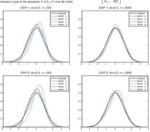
Figure 1. The simulated distributions oft-statistics for the stationary cases.
where
Hωωnst =KE
1/z2
t
(1−β0)2
∞
−∞
1
ω0+π0s2
2
ds×LWd(1,0),
Hθ θnst =E
∂r∗
t (θ0) ∂θ
∂r∗
t (θ0) ∂θ′ ∈R
3×3 .
Note here that the estimators ˆθ and ˆω are asymptotically independent and that the limiting covariance matrix Hθ θnst for the QMLE of θ is nonrandom. Thus, it is only the limiting distribution of ˆωwhich is mixed-normal sinceHωωnstis random.
3.3 Robust Inference
Comparing Theorems 5 and 10, we see that the large-sample distribution of the QMLE changes quite substantially when we move from the stationary case to the nonstationary one. One could therefore fear that, for a chosen regressor, inference would be dependent on whetherxtis stationary or not. However, in both
cases, the limiting distribution of the QMLE is mixed normal with the (possibly random) covariance matrix being the prod-uct of limits of the (appropriately scaled) score and Hessian. Whether xt is stationary or not, a natural estimator of the
co-variance matrix is
ˆ
=Hn−1( ˆϑ)n( ˆϑ)Hn−1( ˆϑ),
where
n(ϑ)= n
t=1 ∂ℓt(ϑ)
∂ϑ
∂ℓt(ϑ)
∂ϑ′ , (19)
and Hn(ϑ) is defined in Equation (10). As we shall see, ˆ
automatically adjusts to the level of persistence and converges to the correct asymptotic limit in both cases. As a consequence, for example, standardt-statistic will be normally distributed in large samples whetherxtis stationary or nonstationary.
-40 -3 -2 -1 0 1 2 3 4
0.1 0.2 0.3 0.4 0.5
DGP 3: dx=0.7, n = 500
normal pdf tstat for α tstat for β tstat for π tstat for ω
-4 -3 -2 -1 0 1 2 3 4
0 0.1 0.2 0.3 0.4 0.5
DGP 3: dx=0.7, n = 5000
normal pdf tstat for α tstat for β tstat for π tstat for ω
-40 -3 -2 -1 0 1 2 3 4
0.1 0.2 0.3 0.4 0.5
DGP 4: dx=1.0, n = 500
normal pdf tstat for α tstat for β tstat for π tstat for ω
-4 -3 -2 -1 0 1 2 3 4
0 0.1 0.2 0.3 0.4 0.5
DGP 4: dx=1.0, n = 5000
normal pdf tstat for α tstat for β tstat for π tstat for ω
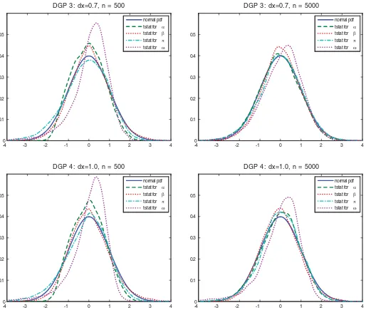
Figure 2. The simulated distributions oft-statistics for the nonstationary cases.
Theorem 11. Under either Assumptions 1–2 or Assumption 3, with ˆdefined in Equation (19),
t :=ˆ−1/2{ϑˆ−ϑ0} →d N(0, I4).
This result shows that standard inferential procedures regard-ing ϑ0 are robust to the persistence ofxt. We conjecture that
similar results hold for other statistics such as the likelihood-ratio statistic.
4. SIMULATION STUDY
To investigate the relevance and usefulness of our asymptotic results, we conduct a simulation study to see whether standard
t-statistics are sensitive toward the level of persistence,dx, in
finite samples. Our simulation design is based on the GARCH-X model with the exogenous regressorxtbeing generated byxt =
(1−L)−dxv
t. The data-generating GARCH parameter values
are set to be ω0=0.01, α0=0.05, β0=0.6, andπ0=0.1. These parameter values are similar to the estimates reported in Shephard and Sheppard (2010), wherex2
t is a realized volatility
measure. The innovation processes{εt}and{vt}are chosen to
be iid standard normal and mutually independent. (We also tried the case forvt = −εtand the results are still similar.) The initial
values are setx0=0 andσ02=0.01.We consider the following four data-generating processes depending ondxinxt:
Stationary cases Nonstationary cases
DGP 1 dx=0.0 DGP 3 dx=0.7
DGP 2 dx=0.3 DGP 4 dx=1.0
The null distributions of each of thet-statistics associated with
ω,α,β,andπare simulated forn=500 and 5000 with 10,000 iterations. The simulation results are reported inFigures 1and2. Figure 1reports the results for the stationary cases and show that the large sampleN(0,1) distribution of thet-statistics is a very good finite-sample approximation. For the nonstationary cases as reported inFigure 2, the asymptoticN(0,1) approximation is also precise, albeit less so compared to the stationary case.
The results for thet-statistic associated withωare consistent with theory. We found that ˆωwill converge toward its limiting distribution at a slower rate compared to ˆθ when the regressor is persistent. This is reflected in the finite-sample distributions of its t-statistic reported in Figures 1 and 2: As persistence grows, the precision of the asymptotic approximation for the distribution ofω’st-statistic deterioriates compared to the other
t-statistics for any given sample size.
Our simulation results show that the empirical distributions of thet-statistics are close to normal for moderate sample sizes and become more so as the sample size increases. This is true regardless of the value of the memory parameter dx inxt. In
conclusion, the individualt-statistics of (ω, α, β, π) are robust toward the dependence structure ofxtin the GARCH-X model.
Researchers do not need to determine whetherxtis stationary or
not before they implement the QMLE and associated inferential tools for the GARCH-X model.
5. CONCLUSION
We have here developed asymptotic theory of QMLEs in GARCH models with additional persistent covariates in the variance specification. It is shown that the asymptotic behavior of the QMLEs depends on whether the regressor is stationary or not. At the same time, standard inferential tools, such as
t-statistics, for the parameters are robust toward the level of per-sistence. In particular, in contrast to the explosive case in pure GARCH models, one can draw inference about the intercept parameterω.
A number of extensions of the theory would be of interest, for example, to show global consistency of ˆωand to analyze the properties of the QMLE in alternative GARCH specifications with persistent regressors.
APPENDIX: PROOFS OF THEOREMS
Proof of Theorem 3. Define ˆϑ∗=arg maxϑ∈×WL∗n(ϑ) where L∗n(ϑ) is defined in Equation (9) withrt(ϑ) given in
Equation (16). We first show consistency of ˆϑ∗ by verifying the conditions in Kristensen and Rahbek (2005, Proposition 2): (i) The parameter space ×W is a compact Euclidean space withϑ0∈×W; (ii)ϑ→ℓ∗t (ϑ) is continuous almost
surely; (iii)L∗
n(ϑ)/n→p L∗(ϑ) :=E[ℓ∗t (ϑ)], where the limit
exists,∀ϑ∈×W; (iv) L∗(ϑ
0)> L∗(ϑ),∀ϑ=ϑ0; and (v)
E[supϑ∈×Wℓ∗t (ϑ)]<+∞. Condition (i) holds by assumption,
while (ii) follows by the continuity of ϑ→r2
t (ϑ) as given
in Equation (16). Condition (iii) follows by the LLN for sta-tionary and ergodic sequences if the limit L∗(ϑ) exists; the
limit is indeed well-defined since ℓ∗
t(ϑ)≤ −log(ω/ω0) such thatE[ℓ∗
t(ϑ)+]<∞. To prove condition (iv), first observe that
rt∗(ϑ0)=1 which in turn implies thatL∗(ϑ0)=0. Moreover, ω0≤log(σ02,t(ϑ0)) such that E[(logσ02,t(ϑ0))−]<∞, while
E[(logσ02,t(ϑ0))+]≤(logE[σ02,ts(ϑ0)])+/s <∞by Jensen’s in-equality and Lemma 2. Thus,E[|ℓ∗t(ϑ0)|]<∞is well defined, while either (a)L∗(ϑ)= −∞or (b)L∗(ϑ)∈(−∞,∞). Now, letϑ=ϑ0be given. Then, if (a) holds,L∗(ϑ0)>−∞ =L∗(ϑ). If (b) holds, the following calculations are allowed:
L∗(ϑ)= −E
log(rt∗(ϑ))+
1
rt∗(ϑ)
−1
εt2
= −E
log(rt∗(ϑ))+
1
r∗
t (ϑ) −
1 ,
where we have used thatE[ε2
t|Ft−1]=1. Thus,L∗(ϑ)≤0= L∗(ϑ0) with equality if and only if r2
t(ϑ)=1 a.s. Suppose
that rt2(ϑ)=1 a.s. ⇔σ02,t(ϑ)=σ02,t(ϑ0) a.s. With ci(θ) :=
(αβi−1, πβi−1)′, we then claim thatω
0=ωandci(θ0)=ci(θ)
for all i≥1; this in turn implies ϑ=ϑ0. We show this by contradiction: Let m >0 be the smallest integer for which
ci(θ0)=ci(θ) (if ci(θ0)=ci(θ) for all i≥1, then ω0=ω). Thus,
a0y2t−m+b0xt2−m=ω−ω0+ ∞
i=1
aiyt2−m−i+
∞
i=1
bix2t−m−i,
where ai :=α0β0i−1−αβ
i−1 and b
i:=π0β0i−1−πβ
i−1. The right-hand side belongs to Ft−m−1 and so a0yt2−m+
b0xt2−m|Ft−m−1 is constant. This is ruled out by Assumption 1(iv). Finally, condition (v) follows from supϑ∈×Wℓ∗t(ϑ)≤
−supϑ∈×Wlog(ω)≤ −log
ω<+∞.
Now, return to the actual, feasible QMLE, ˆϑ. Using Lemma 2,
t−1 <∞ by Berkes, Horv´ath, and Kokoszka (2003, Lemma 2.2) in conjunction with Lemma 1. Thus, supϑ∈|L∗n(ϑ)−Ln(ϑ)|/n=op(1/n). Combining this with
the above analysis ofL∗
n(ϑ), it then follows from Kristensen
and Shin (2012, Proposition 1) that||ϑˆ∗−ϑˆ|| =op(1/n). In
particular, ˆϑis consistent.
Proof of Theorem 5. As shown in the proof of Theorem 3,
||ϑˆ∗−ϑˆ|| =op(1/
√
n); thus, it suffices to analyze ˆϑ∗. The
score and Hessian are given by
Sn∗(ϑ)=∂L
We now verify the two convergence results stated in Equation (11). First, we employ the CLT for martingale differences in Brown (1971, Theorem 2) to show that the first part of Equation (11) holds. By Assumption 1(i),Xt:=∂rt∗(ϑ0)/(∂ϑ){ε2t −1}
is a martingale difference andS∗
n(ϑ0)/√nhas quadratic variation
where we have used Assumption 2(i) and Lemma 4. This shows that Equation (1) in Brown (1971) holds. By station-arity andE[Xt2]<∞,nt=1E[Xt2I{Xt> c√n}]/n=
E[Xt2I{Xt> c√n}]→0, and so Equation (2) of Brown
(1971) also holds.
For the Hessian, ||h∗t (ϑ)|| ≤ {B2,t+B12,t}{1+B0,tεt2} +
B12,tB0,tεt2for allϑin some neighborhood ofϑ0, where the right-hand side has finite first moment; see, for example, Lemma 4. It now follows by standard uniform convergence results for aver-ages of stationary sequences (see, e.g., Kristensen and Rahbek
2005, Proposition 1) that supϑ−ϑ0<δ||H so lies in any arbitrarily small neighborhood w.p.a.1. To com-plete the proof, we verify that Hst
ϑ ϑ(ϑ0) is nonsingular. The process t :=∂σ02,t(ϑ0)/(∂ϑ)∈R4 can be written as t =
βt−1+Wt, whereWt :=[1, yt−1, xt−1, σ02,t−1(ϑ0)]′. Suppose that there existsλ∈R4\ {0}andt ≥1 such thatλ′t =0 a.s.
Sincetis stationary, this must hold for allt. This implies that
λ′W
t =0 a.s. for all t≥1. However, this is ruled out by
As-sumption 1(iv). It must, therefore, hold thatλ′
t/σ02,t(ϑ0)=0 if and only ifλ=0; thus,Hst(ϑ
0)=E[tt′/σ04,t(ϑ0)] is
non-singular.
Proof of Theorem 6. To prove (i), define
ψn′(s)=n−(1/2−d)[ns]
t=1f(xt−1)wt and ψn′′(s)=
n−(1/2−d)[ns]
t=1f(xt−1)E[wt] which both belong to D[0,1].
First, by Theorem 2.1 in Wang and Phillips (2009a), hence-forth WP2009a, and Lemma 1 in Kasparis, Andreou, and Phillips (2012), ψn′′(s)⇒LWd(s,0)×KE[wt]
tributions which together with (i.b) imply weak convergence of
ψ′
Using the covariance condition together with |f(x)| ≤C for someC <∞, we obtain
Billingsley (1974) and wish to show that there exists a sequence ofαn(ǫ, δ) satisfying limδ→0lim supn→∞αn(ǫ, δ)=0 for each
ǫ >0 such that, for 0≤s1≤ · · · ≤sm≤s≤1, s−sm≤δ, we
have
P(|ψn′(s)−ψn′(sm)| ≥ǫ|ψn′(s1), ψn′(s2), . . . , ψn′(sm))
≤ αn(ǫ, δ), a.s. (A.1)
A sufficient conditions for Equation (A.1) is
As before, we first establish a conditional version: Define
αn(Xn, ǫ, δ) as
Similar to the proof of (i.a), we have that, for large enoughn,
αn(Xn, ǫ, δ)
This shows that Equation (A.1) holds in probability conditional onXnwhich in turn implies that it also holds unconditionally ofXn.
arguments as in the proof of part (i) of this lemma,
σu2[ns]
in Proof of Theorem 3.1 in WP2009a, under a suitable probability space there exists an equivalent process xt∗
of xt such that the corresponding quadratic variation
∗n(s)→p Kσu2E[w
of generality we assume that xt satisfies this. We now wish
to show that Vn(s) :=−
is op(1). As before, assuming without loss of
gener-ality qu≤4, E[|
nally, tightness ofVn(s) follows by the same arguments as in
the proof of (i).
Proof of Theorem 9. We first show that θˆ∗ :=
arg maxθ∈L∗n(θ) satisfies ˆθ∗ →P θ0. This is shown by veri-fying conditions (i)–(v) as stated in the proof of Theorem 3. Condition (i) holds by assumption, while (ii) follows by the continuity ofθ→r∗
t (θ) as given in Equation (18). Condition
(iii) follows by the LLN for stationary and ergodic sequences if the limitL∗(ϑ) exists; the limit is indeed well-defined since, by
Lemma 8,E[r∗
t (θ)− k
]<∞for anyk >0. To prove condition (iv), we see that, by the same arguments as in the proof of The-orem 5,L∗(θ0)≥L∗(θ) with equality if and only ifrt∗(θ)=1 spond to the true and model-implied volatility in a pure GARCH model with intercept ˜ω=π/π0. We can then employ the same
Now, return to the original estimator, ˆϑ. Write the log-likelihood as Ln(ϑ)=L∗n(θ)+Rn(ϑ), where Rn(ϑ)=
n t=1[ε
2
t{1/rt∗(θ)−11/rt(ϑ)} +log(rt∗(θ)/rt(ϑ))]/n. Using
the same arguments as in Franq and Zakoian (2012, p. 844) together with Lemma 8, we obtain that Rn(ϑ)=op(1)
uniformly inϑ. Thus, by the same arguments as in the proof of Theorem 3,||ϑˆ −ϑˆ∗|| =op(1) where ˆϑ∗=arg maxθ∈L˜∗n(ϑ)
and ˜L∗
n(ω, θ)=L∗n(θ) for any (ω, θ)∈W×.
Local consistency of ˆωand the local rate result for ˆθ follow as part of the results shown in the proof of Theorem 10 together with Kristensen and Rahbek (2010, Lemma 11).
Proof of Theorem 10. We first establish some
approximations: It follows from Lemma 8 that
βi−1w−2
arguments as in the proof of Lemma 8,
1
1
someδ >0 by the same arguments as in Lemma 8. Similarly, it is easily shown that
We now verify the conditions in Lemmas 11–12 of Kris-tensen and Rahbek (2010) which in turn imply local consis-tency and the claimed asymptotic distribution, respectively. To write our estimation problem in their notation, define
vω,n=n1/4−d/2 and vθ,n=n1/2, so thatVn defined in
Equa-tion (13) can be written as Vn=diag{vω,n, vθ,nI3}. Next, we letQn(ϑ)=Ln(ϑ)/v2ω,ndenote the normalized log-likelihood
and let Un=Vn/vω,n=diag{1, n1/4+d/2I3} be the associated rate matrix. We then claim that
(i) vω,nUn−1
Note that (i) of Equation (A.7) implies that
U−1
We analyze the four elements ofHn(ϑ0) separately. First, using the above approximations,hθ θ,t(ϑ)=hθ θ,t∗ (θ)+op(1),where
t is stationary and geometrically
β-mixing, see, for example, Carrasco and Chen (2002). Since wt and xt are independent and f(x)=1/(ω0+
involvingωare shown to beop(1) in the same manner. Next,
we show (i) of Equation (A.7): Observe that V−1
ing the same arguments as in the proof of Theorem 5 to-gether with the stationary approximation results derived above,
n−1/2S
n,θ(ϑ0)→d N(0, θ θnst). The convergence is joint since
the martingale difference,ε2
t −1, is common to the two
com-ponents of the score, and it is easily checked, by the same arguments as for the hessian, thatωθnst=O1×3.
Finally, we verify Equation (A.8): We have already proved that this holds for Hn,θ θ(ϑ). What remains is to show that it
also holds for the components involvingω. We only show the result for∂2Qn(ϑ)/(∂ω2) since the proof for the other partial
derivatives follows along the same lines. For ϑ ∈Bn(ϑ0, ǫ),
θ−θ0 ≤n−1/4−d/2ǫandω−ω0 ≤ǫ. Thus, by the mean-value theorem, for some ¯ϑ on the line segment connecting ϑ
andϑ0,
Employing the same arguments as in the analysis of the Hessian,
we obtain the desired result.
Proof of Theorem 11. For both the stationary and
nonsta-tionary case, we have already shown as part of the proofs of Theorems 5 and 10 that supUn(ϑ−ϑ0)<δ||V
on the right-hand side is continuous w.r.t. ϑ and, by Lemma 4, is uniformly bounded by a stationary sequence with sec-ond moment. It, therefore, follows by the uniform LLN, that supϑ−ϑ0<δ||n(ϑ)/n−
For the nonstationary case, we proceed as in the analysis of the Hessian: First, write
approximation, and so, similar to the stationary case, we can appeal to a uniform LLN for stationary and ergodic sequences to obtainn,θ θ( ˆϑ)/n→p nst. Next,
and, similar to the proof of Equation (A.8), supUn(ϑ−ϑ0)<δn
The online supplementary material contains proofs of lem-mas.
ACKNOWLEDGMENTS
This article benefited from discussions with Joon Y. Park, Peter Phillips, Anders Rahbek, and Qiying Wang. We also wish to thank participants at seminars at University of Not-tingham, the NBER-NSF time series conference 2012 at Texas A&M, and a time series workshop at University of Copenhagen for comments and suggestions. Kristensen gratefully acknowl-edges financial support from the European Research Council through a starting grant (No 312474), Economic and Social Re-search Council through the ESRC Centre for Microdata Meth-ods and Practice grant RES-589-28-0001, and the Danish Re-search Council through its funding of CREATES. This work was supported by a grant from the Kyung Hee University (KHU 2012-1676).
[Received May 2012. Revised January 2014.]
REFERENCES
Barndorff-Nielsen, O. E., and Shephard, N. (2007), “Variation, Jumps and High Frequency Data in Financial Econometrics,” inAdvances in Economics and Econometrics. Theory and Applications, Ninth World Congress, eds. R. Blundell, T. Persson, and W. K. Newey, Econometric Society Monographs, Cambridge, UK: Cambridge University Press, pp. 328–372. [416] Berkes, I., Horv´ath, L., and Kokoszka, P. (2003), “GARCH Processes: Structure
and Estimation,”Bernoulli, 9, 201–227. [425]
Billingsley, P. (1974), “Conditional Distributions and Tightness,”Annals of Probability, 2, 480–485. [425]
Bollerslev, T. (1986), “Generalized Autoregressive Conditional Heteroskedas-ticity,”Journal of Econometrics, 31, 307–327. [416]
Bollerslev, T., and Melvin, M. (1994), “Bid-Ask Spreads and the Volatility in the Foreign Exchange Market: An Empirical Analysis,”Journal of International Economics, 36, 355–372. [416]
Brenner, R. J., Harjes, R. H., and Kroner, K. F. (1996), “Another Look at Models of the Short-Term Interest Rate,”Journal of Financial and Quantitative Analysis, 31, 85–107. [416]
Brown, B. (1971), “Martingale Central Limit Theorems,”Annals of Mathemat-ical Statistics, 42, 59–66. [425]
Carrasco, M., and Chen, X. (2002), “Mixing and Moment Properties of Various GARCH and Stochastic Volatility Models,”Econometric Theory, 18, 17–39. [427]
Dittmann, I., and Granger, C. W. J. (2002), “Properties of Nonlinear Trans-formations of Fractionally Integrated Processes,”Journal of Econometrics, 110, 113–133. [418]
Dominguez, K. (1998), “Central Bank Intervention and Exchange Rate Volatil-ity,”Journal of International Money and Finance, 17, 161–190. [416] Engle, R. F. (2002), “New Frontiers for ARCH Models,”Journal of Applied
Econometrics, 17, 425–446. [416]
Engle, R. F., and Gallo, G. M. (2006), “A Multiple Indicators Model for Volatility Using Intra-Daily Data,”Journal of Econometrics, 131, 3–27. [416] Escanciano, J. M. (2009), “Quasi-Maximum Likelihood Estimation of
Semi-Strong GARCH Models,” Econometric Theory, 25, 561–570. [420]
Fleming, J., Kirby, C., and Ostdiek, B. (2008), “The Specification of GARCH Models With Stochastic Covariates,”Journal of Futures Markets, 28, 911– 934. [416]
Franq, C., and Zako¨ıan, J.-M. (2012), “Strict Stationarity Testing and Estimation of Explosive and Stationary Generalized Autoregressive Conditional Het-eroskedasticity Models,”Econometrica, 80, 821–861. [417,419,421,426] Gallo, G., and Pacini, B. (2000), “The Effects of Trading Activity on Market
Volatility,”European Journal of Finance, 6, 163–175. [416]
Girma, P., and Mougoue, M. (2002), “An Empirical Examination of the Relation Between Futures Spreads Volatility, Volume, and Open Interest,”Journal of Futures Markets, 22, 1083–1102. [416]
Glosten, L. R., Jagannathan, R., and Runkle, D. (1983), “On the Relation Be-tween the Expected Value and the Volatility of the Nominal Excess Return on Stocks,”Journal of Finance, 48, 1779–1801. [416]
Gray, S. F. (1996), “Modeling the Conditional Distribution of Interest Rates as a Regime-Switching Process,”Journal of Financial Economics, 42, 27–62. [416]
Hagiwara, M., and Herce, M. (1999), “Endogenous Exchange Rate Volatility, Trading Volume and Interest Rate Differentials in a Model of Portfolio Selection,”Review of International Economics, 7, 202–218. [416] Hall, P., and Heyde, C. C. (1980),Martingale Limit Theory and Its Application,
New York: Academic Press. [426]
Han, H. (2014), “Asymptotic Properties of GARCH-X Processes,” forthcoming inJournal of Financial Econometrics. [417,418]
Han, H., and Park, J. Y. (2012), “ARCH/GARCH With Persistent Covari-ates: Asymptotic Theory of MLE,”Journal of Econometrics, 167, 95–112. [417,421]
——— (2013), GARCH With Omitted Persistent Covariate, unpublished manuscript, Kyung Hee University. [417,421]
Hansen, P. R., Huang, Z., and Shek, H. H. (2012), “Realized GARCH: A Complete Model of Returns and Realized Measures of Volatility,”Journal of Applied Econometrics, 27, 877–906. [416]
Hodrick, R. (1989), “Risk, Uncertainty, and Exchange Rates,”Journal of Mon-etary Economics, 23, 433–459. [416]
Hwang, S., and Satchell, S. E. (2005), “GARCH Model With Cross-Sectional Volatility: GARCH-X Models,”Applied Financial Economics, 15, 203–216. [416]
Heber, G., Lunde, A., Shephard, N., and Sheppard, K. (2009),OMI’s Realized Library, Version 0.1, Oxford-Man Institute, University of Oxford. [417] Jensen, S. T., and Rahbek, A. (2004), “Asymptotic Inference for Nonstationary
GARCH,”Econometric Theory, 20, 1203–1226. [417,419,420]
Kasparis, I., Andreou, E., and Phillips, P. C. B. (2012), “Nonparametric Predic-tive Regression,” unpublished manuscript, University of Cyprus. [425] Kristensen, D., and Rahbek, A. (2005), “Asymptotics of the QMLE for a Class of
ARCH(q) Models,”Econometric Theory, 21, 946–961. [417,420,424,425] ——— (2010), “Likelihood-Based Inference for Cointegration With Nonlinear
Error-Correction,”Journal of Econometrics, 158, 78–94. [422,426,427] Kristensen, D., and Shin, Y. (2012), “Estimation of Dynamic Models With
Nonparametric Simulated Maximum Likelihood,”Journal of Econometrics, 167, 76–94. [425]
Lamoureux, C. G., and Lastrapes, W. D. (1990), “Heteroskedasticity in Stock Return Data: Volume Versus GARCH Effects,”Journal of Finance, 45, 221–229. [416]
Marsh, T. A., and Wagner, N. (2005), “Surprise Volume and Heteroskedasticity in Equity Market Returns,”Quantitative Finance, 5, 153–168. [416] Park, J. Y., and Phillips, P. C. B. (1999), “Asymptotics for Nonlinear
Trans-formations of Integrated Time Series,”Econometric Theory, 15, 269–298. [418]
Shephard, N., and Sheppard, K. (2010), “Realising the Future: Forecasting With High Frequency Based Volatility (HEAVY) Models,”Journal of Applied Econometrics, 25, 197–231. [416,424]
Wang, Q. (2013), “Martingale Limit Theorem Revisited and Nonlinear Cointe-grating Regression” forthcoming in,Econometric Theory. [421]
Wang, Q., and Phillips, P. C. B. (2009a), “Asymptotic Theory for Local Time Density Estimation and Nonparametric Cointegrating Regression,” Econo-metric Theory, 25, 710–738. [418,419,421,425]
——— (2009b), “Structural Nonparametric Cointegrating Regression,” Econo-metrica, 77, 1901–1948. [418]
Yoshihara, K. (1976), “Limiting Behaviour of U-Statistics for Stationary, Ab-solutely Regular Processes,”Zeitschrift f¨ur Wahrscheinlichkeitstheorie und verwandte Gebiete, 35, 237–252. [421]