10 (2000) 257 – 273
Size effect, book-to-market effect, and survival
Xiaozu Wang *
Department of Economics and Finance,City Uni6ersity of Hong Kong, Hong Kong
Received 15 July 1999; accepted 12 April 2000
Abstract
Previous studies find that small stocks have higher average returns than large stocks, and
the difference between the returns can not be accounted for by the systematic risk,b. In my
analysis of Compustat and CRSP data from 1976 to 1995, and simulation experiments based on the data, I find the size effect can be largely explained by data truncation that is caused by survival. Small stocks’ returns are more volatile, and small stocks are more likely to go bankrupt and less likely to meet the stock exchanges’ minimum capitalization requirements for listing. As a result, they are more likely to drop out of the sample. Including small stocks that do well and excluding those that do poorly, ex post, gives rise to higher returns for small-size portfolios. I conclude that the size effect is largely a spurious statistical inference resulting from survival bias, not an asset pricing ‘anomaly’. © 2000 Elsevier Science B.V. All rights reserved.
JEL classification:G12; G14
Keywords:Asset pricing anomalies; Survival bias; Size effect
www.elsevier.com/locate/econbase
1. Introduction
Two accounting variables, market value of equity (ME, measured as the product of the shares outstanding and the price of a stock) and ratio of book-to-market value of equity (BM), are found to have a predictive power on stock returns. Among others, Fama and French (1992) (FF) and Lakonishok et al. (1994) (LSV) find that in a long run, the average returns of small ME stocks are higher than
* Tel.: +852-27887407; fax: +852-27888806.
E-mail address:[email protected] (X. Wang).
those of large ME stocks (known as the size effect), and the average returns of high BM stocks are higher than those of low BM stocks (the BM effect). FF also found that only a very small portion of the difference in returns can be accounted for by
b, the systematic risk. These findings reject CAPM, which asserts that: (1) there is
a positive, linear relationship between the stock’s expected returns and itsband (2)
bis sufficent to explain the cross-section of stock returns. Furthermore, by showing
that public information, ME and BM, can help to predict stock returns, these
findings seem to undermine the efficient market hypothesis1.
Since the size and BM effect are not consistent with CAPM, they are considered asset pricing anomalies. Although they have been received with some skepticism
among academics2
, the results seem to remain fairly robust3
. Asset pricing anoma-lies suggest that one can beat the market, probably without adding to risk, by investing in stocks with a low ME or high BM, so they have been quickly embraced by practitioners.
In this paper I address the possible data truncation bias in ‘anomaly’ studies that is caused by survival. In anomaly studies and empirical analysis of stock returns in general, a stock’s return can be calculated only if it survives the period of interest, which may vary from a few months to a few years. Since firms that perform well are more likely to survive and remain in the sample than those that perform poorly, the observed returns of surviving firms tend to be biased upward. I call this survival bias. When portfolios are formed by sorting stocks according to ME or BM, survival bias can be particularly acute for portfolios of small ME stocks or high BM stocks. In these cases, stocks are more likely to drop out because of both small
size and high b-risk, resulting in high average returns for portfolios with small
stocks or high BM stocks.
It is important to note that the survival bias discussed here is not the same as discussed by Fama and French (1996), Kothari et al. (1994) or Chan et al. (1995). Their concern is that, especially before the mid 1970s, Compustat is biased towards bigger and maturer firms by not including younger and smaller firms. This type of bias does not exist in CRSP since it includes virtually all the firms that have been traded on the NYSE and AMEX since 1926. But in terms of my study, survival bias exists even in CRSP simply because we only observe the return series up to the point when a firm ceases to survive and the reason for a firm not surviving may often be correlated with its performance prior to the point of dropout. In this sense, the survival bias that I discuss here is a type of data truncation rather than data selection, is intrinsic to the time series of stock returns and can not be amended by changing the data collection process.
1Methods to estimatebused in previous papers may be subject to debate, but these are beyond the
scope of this paper. Because my results only depend on the empirical fact that small stocks and high book-to-market stocks have higher systematic, as well as total risk, the precision of estimatedbshould not change my results.
Using data and an experimental design similar to that used by FF and LSV, I conducted simulation experiments, and found that survival explains a significant portion of the size effect and a smaller portion of the BM effect. With a very simple rule for survival that is based on limited liability and a very modest average number of firms dropping out each year, I am able to show that the the cross-section
returns of size portfolios generated by a CAPM model can exhibit a size effect4and,
to a lesser extent, a BM effect. For example, with an average of about 3% of the firms dropping out from the cross-section each year, the average annual returns of a portfolio consisting of the smallest 10% of the stocks rises to 21.3%, in contrast to the 19.9% predicted by CAPM, the portfolio of the 10% highest BM stocks rise to 18.8%, in contrast to the 18.5% predicted by CAPM.
My main findings are as follows. First, size effect is largely a result of data truncation that is caused by survival. It is, at least partly, a spurious statistical inference rather than an asset pricing anomaly. Second, since BM is a scaled measure of ME, the BM effect can also be partly attributed to survival. Third, when size is controlled for, the cross-section variation of returns of BM-based portfolios largely disappears, except within the smallest ME portfolio. Moreover, I find the BM effect much weaker than suggested in previous studies.
2. The possibility of survival bias: some empirical evidence
A few explanations have been provided for the size effect and BM effect ‘anomalies’5
. The first, offered by FF, is that small stocks have higher systematic
risk, and part of that risk is not captured by market b. The second explanation,
‘data snooping’, is offered by Lo and MacKinlay (1990). The third explanation is data selection bias resulting from Compustat data collection procedures, as offered by Ball et al. (1995). The fourth explanation is that market overreacts because of judgment bias based on psychological and institutional reasons (Thaler, 1993; Lakonishok et al., 1994). The last reason, offered by Berk (1995), argues that ‘size will in general explain the part of the cross-section of expected returns left unexplained by an incorrectly specified asset pricing model’.
The possible role of data truncation that is caused by survival has received little attention in explaining the size effect and BM effect. As Brown et al. (1992) show in their study of mutual fund performance, survival bias can be substantial. The anomaly studies and empirical analysis of rates of return in general, are implicitly conditional on security surviving in the sample. Such conditioning ‘induces a spurious relationship between observed return and total risk for those securities that survive to be included in the sample’ (Brown et al., 1995, p. 853).
4The size effect puzzle has two parts. Compared with what is predicted by CAPM, small stocks’
average returns are too high and large cap stocks’ average returns are too low. I only address the small cap part of the puzzle in this paper.
In my sample, as in previous anomaly studies, a stock must have a continuous trading record and keep the same identity in order to survive, and it may fail to survive for quite complex reasons. An incomplete list of reasons includes bankruptcy, merger and acquisition, liquidation, exchange switch, failure to meet the requirements set by the stock exchange or SEC, and going private. Table 1 shows the reasons stocks drop out of the NYSE and AMEX. In the NYSE, from 1926 to 1995, 4989 stocks were listed, and about 48% of them, 2391, subsequently dropped out. In AMEX, from 1962 to 1995, about 72% of the stocks that had been listed were subsequently delisted. More than half of the dropouts result from mergers (the first row) and about 30% from liquidation or failure to meet the listing requirement set by the exchanges (the third and fourth row). Similar patterns hold
for my NYSE – AMEX sample from 1975 to 19956. I should note that the actual
percentage of firms that drop out as a result of business failure is higher than 30% because many of those that merged or were acquired were poor performers. As found by Mørck et al. (1988), takeover targets, especially in cases of hostile takeover, often have significantly lower Tobin’s q. Although I do not have detailed information on why firms were acquired or merged in CRSP, it seems reasonable to assume that more than half of the cases were due to poor performance, as about half of the sample from Mørck et al. (1988) is categorized as hostile takeovers.
Table 1
Reasons for data attrition in NYSE–AMEX: 1926–1995a
Reason for delisting NYSE 1926–1995 AMEX 1962–1995 NYSE–AMEX 1975–1995
Firms % Firms % Firms %
63.36
Merger 1515 1028 52.00 1727 62.89
Exchange switch 213 8.91 165 8.35 298 10.85
96
Delisted by the exchange 524 688 34.80 611 22.25
37 1.54 15
aA stock is identified by its CUSIP and is considered delisted if the return series was ended before
December 31, 1995. The first column lists the reason for a firm to drop out of CRSP. The last row shows the total number of firms that drop out during the period. Percentages are calculated with regard to the total number of firms that drop out of CRSP during the period. Data cover all NYSE and AMEX stocks corresponding to the time period as shown in the Table. I break the data into three periods. The first period corresponds to the complete time span in CRSP. The second covers the period since the inception of AMEX. The third corresponds to the data that I use in my study. Comparing the three periods I find that the percentage of firms that drop out in each category remains stable over the years.
6When comparing the last two rows of columns 2, 4 and 6, I find the number of firms that do not
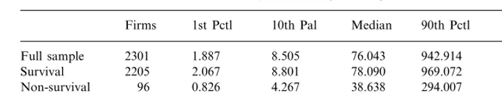
Table 2
Cross-section of size: NYSE–AMEX stocks, 1962–1995 (million $)a
Firms 1st Pctl 10th Pal Median 90th Pctl 99th Pctl
Full sample 2301 1.887 8.505 76.043 942.914 6048.908 8.801 78.090 969.072
Bankruptcy 26 0.814 1.676 10.042 85.466 316.707
aThe table shows the time series averages of the cross-section of size. To avoid the ‘January effect’,
I calculate the size at the end of each April as the product of shares outstanding and the closing price. The time period is selected so as to coincide with the inception of AMEX and to be comparable with the data used by FF and LSV. A firm is considered a survivor if its return series is available through the end of the following April and a non-survival otherwise. Among non-survivals, I also identify firms that drop out as a result of bankruptcy. I calculate the 1st, 10th, 50th, 90th and 99th percentiles of size for each cross-section, and the time averages for these are shown in columns 3–7.
Small stocks are less likely to survive for at least two reasons. The first is financial. The low market value of equity may simply reflect the firm’s poor cash flow, which in turn may lead to bankruptcy when the firm can not meet its debt payment or other kinds of liabilities. Small firms are also more vulnerable to ‘credit crunch’ than bigger firms, especially during an economic downturn. The second reason is institutional. Even if the firm is fully equity-financed and has no problem in meeting its liabilities, when the market value of its equity, or its stock price is too low, the stock exchange may decide to halt trading in the stock or delist it because the stock does not meet the minimum listing requirements. Small stocks are more vulnerable to this type of delisting.
The likelihood that a small stock will drop out of the sample is exacerbated by its high total risk, which includes its systematic risk, b, as well as the residual risk, measured by the residual term in the regression of the stock returns on market
index returns. It is an empirical fact that small stocks have both high b and high
residual risk. As reported by FF, the correlation between b and the natural log of
equity than survival firms, listed in the second row, with the median size of the non-survival being less than half of that of the survival. The non-survival firms that go bankrupt, listed in the last row, are even smaller, with the median size of the bankrupted firms being less than one-fifth of that of the survival firms. The evidence suggests that market capitalization is a crucial factor that affects whether a stock will remain in CRSP.
The fact that small stocks are more likely than large stocks to drop out of CRSP presents a problem for research on long-term stock returns. The problem is particularly severe for anomaly studies for two reasons. First, previous anomaly studies typically group small stocks into one portfolio, which presumably will suffer most of the attrition in the cross-section. Second, anomaly studies usually require a stock to have a 2 – 5 year return series. In a period of such length, accumulated data attrition can be substantial.
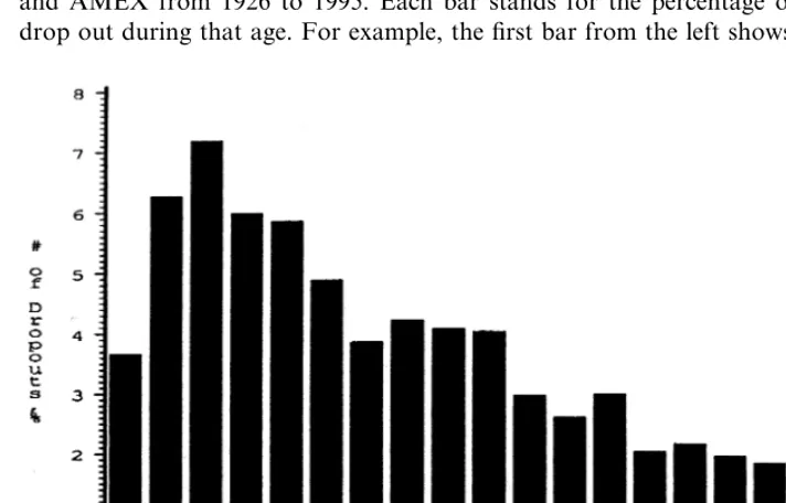
Fig. 1 illustrates long-term survival of NYSE – AMEX stocks, from 1926 to 1995.
The x-axis indicates the number of years that a stock has been listed or a firm’s
‘age’ by the time it drops out of the NYSE – AMEX. The y-axis stands for the
number of firms that drop out as a percentage of total firms that are listed in NYSE and AMEX from 1926 to 1995. Each bar stands for the percentage of firms that drop out during that age. For example, the first bar from the left shows that about
3% of the firms drop out within 1 year of being listed, and the second bar from the left shows that about 7% of all the firms survive the first year but drop out during the second year after being listed. In other words, each bar represents the
probabil-ity that a firm will drop out at age t conditional on its survival t−1 years in the
sample. Nearly 10% of the firms drop out within the first 2 years after they are listed, and nearly 17% within the first 3 years. Nearly 30% of the stocks drop out within the first 5 years. The probability of survival increases with the number of years that the stock has already survived7. Given the substantial data attrition, the
effect of survival on observed returns should be checked rather than just assumed.
3. Method
The primary data sources used for this study are the annual industrial series of Compustat and the monthly stock file of the CRSP (Center for Research of Security Prices at the University of Chicago). The sample universe is the NYSE and AMEX non-financial firms, and the sample period for my study is 1975 – 1994. The sample period and universe of stocks in my study roughly represent an intersection of Fama and French (1992) and Lakonishok et al. (1994). Following LSV’s design, I form portfolios based on ME and BM at the end of each April to mitigate the ‘January effect’ and make sure most firms’ fourth quarter accounting information is available to the public by the time of portfolio formation. ME and BM data are taken from the fourth quarter of the most recent fiscal year.
We test the effect of survival on cross-section of returns using the following simulation experiment.
First, I randomly draw a sample of 250 stocks with replacement from one cross-section of CRSP-Compustat. For each stock in the sample, a one year buy-and-hold return is simulated by assuming that the return process follows CAPM and no dividend is paid during the holding period. In particular, we assume the following return process for each stock:
rit=rf+bitxt+sitit
where rf is the risk-free rate and assumed to be 0.07 per annum8, b
it is the b of
stock i in year t, xt is the risk premium of year t, assumed to be normally
distributed with mean 0.086 and standard deviation 0.208,sitis the residual risk of
stockiin yeart, itis the standard normal deviate and is assumed i.i.d. across firms and over time.
bit and sit for each stock are estimated each year at the end of December,
immediately before the portfolio formation, provided that there are 60 months or more prior return data available and the estimates are used in the simulation for
7This is consistent with the dynamics of firm growth found by Mansfield (1962), namely the likelihood
of failure decreases with a firm’s age.
year t+1. The market model is used to estimate bit and sit by regressing stock
returns on the returns of the market portfolio in the same period. Sixty months of data are required and the equally-weighted market return in CRSP is used as a proxy for market return. Estimates are deemed to be reasonably accurate and kept
if the market model regression has adjustedR2]0.05. Each year, there are between
5 and 10% estimates discarded for this reason. The results I report here are not
sensitive to whether all estimates of b are kept or not.
Since about 30% of NYSE – AMEX firms do not survive 60 months in the data,
I can not estimate bfor these firms. But these firms are used in Fama and French
(1992) and Lakonishok et al. (1994), and tend to be small and important for my study. Therefore I obtain estimates of bit and sit for these stocks by inferring bit
based on the estimated relation between ME and bit, and sit on the relation
between bit andsit
9
.
Then I form portfolios by grouping stocks according the their associated ME, BM or both ME and BM. Ten ME portfolios are formed by sorting stocks according to ME, the first one containing 25 stocks with the smallest ME and the tenth contains the 25 stocks with the highest ME. Ten BM portfolios are formed by sorting stocks according to BM, with the first BM portfolio containing the 25 stocks with the lowest BM and the tenth containing the highest. I then form 100 ME-BM portfolios by sorting stocks according to both ME and BM, indepen-dently. The intersection of ME and BM portfolios becomes the ME-BM portfolio.
On a plane where ME is the x-axis and BM is the y-axis, each stock can be found
according to its associated ME and BM values. For example, if a stock falls in the first ME portfolio and in the second BM portfolio, it belongs to ME – BM portfolio (1, 2). Since ME-BM portfolios result from sorting by ME and BM, independently, each portfolio may not have the same number of stocks. For example, since ME and BM are negatively correlated, the highest-ME-lowest-BM portfolio contains more stocks than the highest-ME-highest-BM portfolio.
We calculate the portfolio returns in two ways. A simple average of each stock included at the time of portfolio formation, equally-weighted by each stock, gives the portfolio return, which I call the portfolio return without attrition.
Then, I calculate the portfolio return with attrition. The attrition rule is based on the fact that small stocks are more likely to drop out of the sample. If the market
value of equity is below the ‘threshold’ in year+1, the firm is excluded. For each
year from 1975 to 1994, I choose a ‘threshold’ such that there is on average an approximate 3% dropout from the section, which matches what I observe in CRSP. The ‘threshold’ rises from 1975 to 1994, and the average is US$3 million, which conforms closely with the stock exchange minimum listing requirement. For
9The relationship between b and size is estimated by running a cross-sectional OLS regression:
Fig. 2. The average returns of size-based portfolios: with and without survival attrition. The size portfolios are formed in the way described in the text. The black line represents the annual return generated by a CAPM model and the grey line represents the return when there is attrition. Thex-axis stands for ten size portfolios, where portfolio 1 contains the smallest stocks, and portfolio 10 contains the largest stocks. The portfolio return is a simple average of associated stock returns, each stock receiving equal weight. The simulation is run for each cross-section of 250 stocks randomly drawn from Compustat-CRSP data and is repeated 1000 times.
example, in 1994 the minimum listing market capitalization requirement was US$5 million on the NYSE and US$3 million on AMEX (New York Stock Exchange, 1994).
For each simulation date, I compute returns for each ME, BM, ME-BM portfolio, with and without attrition. I repeat the process 1000 times so that I can observe the distribution of the cross-section of returns. By comparing the cross-sec-tion of returns before and after any data attricross-sec-tion, I can assess the survival effect. Since the return series are generated by CAPM, any inconsistency between return without attrition and with attrition must be caused by survival.
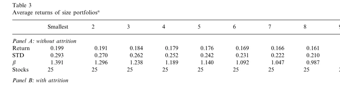
4. Major findings
Fig. 2 shows my main findings by contrasting the cross-section returns of size portfolios without data attrition (represented by the black line with crosses) and with attrition (represented by the grey line). In the figure, the x-axis represents the
ten size portfolios and they-axis shows their returns. Attrition has a marked effect
portfolios. This is an obvious consequence of the adjustment of the return of the smallest-size portfolio after the attrition rule is applied to the data.
More detailed results are shown in Table 3. Without attrition (panel A) the smallest portfolio has a return of 19.9%. When an attrition is applied to the data and, on average, about 3% of the cross-section drop out each year (panel B), the 1-year buy-and-hold return of the smallest-size portfolio deviates from the CAPM prediction and rises from 19.9 to 21.3%. Simultaneously, the standard deviation of
returns of the smallest-size portfolio drops, and so does the average b of stocks in
the portfolio. In other words, conditional on survival, the observed return is higher than that predicted by CAPM, and observed systematic risk and total risk are lower than those calculated before some stocks dropped out. Overall this leads to an overestimate of the risk premium associated with small stocks, which then results in rejection of CAPM.
The effects of survival on book-to-market portfolios shown in Table 4 are less marked than those on size portfolios. With attrition, the returns of the highest BM portfolio rise by 0.3%. While the size effect in my simulation is similar to that found by FF, my book-to-market effect is much less significant than theirs.
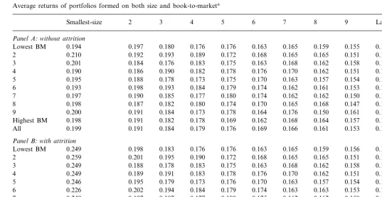
My last finding is that after firm size is controlled, there is very little variation in returns across BM portfolios. This is different from what was found by FF and LVS, but consistent with some recent studies. For example, Loughran (1997) found that ‘within the largest size quintile, book-to-market had no reliable predictive power’. In Table 5, the rows give the size of portfolio returns, given the book-to-market value of the stocks, while columns give BM portfolio returns, given the stocks’ size. For example, the first row shows the cross-section average return variation of size portfolios for stocks that have book-to-market value below the 10th percentile of the cross-section. Although there is some cross-section variation across the BM portfolios, as shown in the last column, this variation largely disappears when size is controlled for, as is apparent from columns 2 to 11. This is so both with (panel B) and without (panel A) data attrition. When there is attrition, the cross-section variation of BM portfolios is concentrated in the smallest-size
decile (first column in panel B)10. Table 5 separates the role of size from BM and
gives a better description of the cross-section variation of stock returns. It suggests
that the BM effect in part may be a variation of the size effect. Because I infer b
and residual risk of firms that I don’t have 60 months of returns and I use an attrition rule that only depends on size, these results are probably only suggestive. Further studies are needed to establish these results as empirical regularities.
5. A brief note on Lakonishok et al. (1994)
It is probably helpful to relate my findings to Lakonishok et al. (1994). Using the data provided in the working paper version of their paper, I carry out a simulation
10The fact that the smallest-size and lowest BM portfolio has the highest return should be discounted
Wang
Average returns of size portfoliosa
Smallest 2 3 4 5 6 7 8 9 Largest
Panel A:without attrition
0.169
Return 0.199 0.191 0.184 0.179 0.176 0.166 0.161 0.153 0.144
0.231 0.222 0.210 0.195 0.176
0.242 0.293
STD 0.270 0.262 0.252
1.140
1.391 1.296 1.238 1.189 1.092 1.047 0.987 0.916 0.809
b
Stocks 25 25 25 25 25 25 25 25 25 25
Panel B:with attrition
0.170 0.166 0.161
0.193 0.153
Return 0.213 0.185 0.180 0.176 0.144
0.251 0.241 0.230 0.222 0.209 0.194 0.175
0.269
STD 0.278 0.261
b 1.360 1.293 1.240 1.188 1.140 1.092 1.047 0.987 0.915 0.809
25 25 25 25 25
24.936 24.546 24.889 24.928
Stocks 17.385
aThe portfolios are formed on the basis of size in the way described in the text, and the return for each stock is generated by CAPM. Panel A contains
X
Average returns of book-to-market portfoliosa
5
Smallest 2 3 4 6 7 8 9 Largest
Panel A:without attrition
0.171 0.173
Return 0.169 0.167 0.167 0.169 0.167 0.174 0.180 0.185
0.230 0.236 0.233 0.251 0.254
0.229 0.228
STD 0.222 0.224 0.169
1.077
1.068 1.043 1.057 1.073 1.087 1.110 1.139 1.186 1.254
b
Return 0.169 0.167 0.170 0.168 0.188
0.170 0.227 0.228 0.233 0.230 0.247 0.245
0.220
STD 0.226 0.222
1.071
1.059 1.036 1.051 1.067 1.081 1.103 1.131 1.173 1.227
b
24.541 24.407 24.338 23.809 21.258 24.575
24.602 24.554 Stocks 24.202 24.566
aSimilar to Table 3. The column headed ’Smallest‘ represents the portfolio of stocks with the smallest BM value and the one headed. ‘Largest’ represents
X
Average returns of portfolios formed on both size and book-to-market
6 7 8 9 Largest-size All
Smallest-size 2 3 4 5
0.189 0.172 0.168 0.165 0.165 0.151 0.144 0.167
2 0.210 0.192 0.193
0.190 0.186 0.190 0.182 0.176 0.170 0.162 0.151 0.143 0.169
4
0.173 0.175 0.170 0.163 0.157 0.154 0.141 0.167
5 0.195 0.188 0.178
0.197 0.190 0.185 0.177 0.174 0.162 0.162 0.150 0.150 0.173
7
0.170 0.165 0.168 0.147 0.148
8 0.198 0.187 0.182 0.180 0.174 0.174
0.164 0.176 0.150 0.161 0.143
0.178 0.180
0.200
9 0.191 0.184 0.173
0.169
0.198 0.191 0.182 0.178 0.162 0.168 0.164 0.157 0.159 0.185
Highest BM
0.169
All 0.199 0.191 0.184 0.179 0.176 0.166 0.161 0.153 0.144 –
Panel B:with attrition
2 0.259 0.201 0.195 0.190 0.172 0.145 0.168
0.163 0.168 0.162 0.158 0.140
0.175 0.167
3 0.249 0.188 0.178 0.183
0.183 0.178 0.176 0.170 0.162 0.151 0.143 0.170 0.189
0.226 0.202 0.194 0.184 0.174 0.163 0.163 0.153 0.148 0.172
6
0.177 0.180 0.175 0.162 0.162 0.150 0.150 0.174
7 0.249 0.197 0.187
0.223 0.193 0.184 0.173 0.164 0.176 0.150 0.161 0.143 0.181
9
0.162 0.168
Highest BM 0.215 0.193 0.183 0.178 0.169 0.164 0.157 0.159 0.188
0.170 0.166 0.161 0.153 0.144 –
0.176 0.180
0.185 0.193
All 0.213
aPanel A presents the simulated return without attrition and Panel B with attrition. In each panel, 100 portfolios are formed by sorting stocks
experiment as described in the previous section, and the results point to a strong possibility of survival bias in the BM effect reported in that paper.
My simulation experiment is similar to that described in Section 3, except that in
this case, I use the estimates of average residual risk and b risk of BM portfolios
from Lakonishok et al. (1994). In addition, I assume there are 100 stocks in each of the ten BM portfolios. I also assume that stocks in the same portfolio have the
same residual risk andbrisk, which are equal to the portfolio averages. The annual
returns are then generated for each stock by assuming the return process follows CAPM, and the portfolio returns are calculated as a simple average of returns of stocks that ‘survive’. This is equivalent to assuming the dropout stocks’ returns are equal to the portfolio average, as LSV did in their paper. The simulation is carried out 50 000 times.
We apply the simplest survival rule to the sample. In each of the simulations, a
stock will not survive if its return falls into the bottom X% of the cross-section of
1000 stocks. By comparing the cross-section of returns before and after attrition, I can access the survival effect.
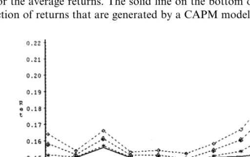
Fig. 3 shows the cross-section of returns of BM portfolios with and without
survival, where the x-axis represents the order of BM portfolios and the y-axis
stands for the average returns. The solid line on the bottom of the graph shows the cross-section of returns that are generated by a CAPM model without any attrition.
The other three dashed lines represent the cross-section of returns when 1, 3 and 5% of the stocks with the lowest returns drop out, respectively. The most noticeable changes in average returns as a result of attrition occur with the highest BM portfolio. Changes to low BM portfolios are much less significant. For example, when stocks with returns in the bottom 3% drop out of the sample, the average return of the highest BM portfolio rises to more than 20% per annum from 16.5% (provided there is no attrition and I include all stocks in calculating the average portfolio returns). In the meantime, returns of low BM portfolios increase by a much smaller amount. The observed cross-section of returns deviates from the underlying CAPM process and exhibits a book-to-market effect simply becaue of survival bias. This raises doubts about LSV’s findings on the BM effect and suggests a significant part of the puzzle may be explained by survival bias.
6. Conclusions
In this paper, I have demonstrated that survival alone can cause the size effect and book-to-market effect. Abnormal returns of small size and high book-to-mar-ket stocks can be observed even when CAPM holds perfectly, solely because the stock returns are truncated from below, and such truncation is much more likely to occur in portfolios consisting of small or high book-to-market stocks.
The results in this paper suggest three propositions. First, survival is largely responsible for the size effect by raising the average returns of the smallest size portfolio. Second, the high average returns associated with the highest BM portfo-lio can also be partly attributed to survival bias. Third, after size is controlled for, BM has little correlation with returns, which suggests that the BM effect in part may be a variation of size effect. While the first two propositions are my explanations of previous findings, the last is a new finding that calls for further investigations.
These findings throw light on some other size-related anomalies, in which a set of accounting variables are found to have predictive power on returns. The better known among these include the price – earnings ratio, and cash flow to market equity ratio (Lakonishok et al., 1994).
These findings are consistent with some recent studies on asset pricing anomalies. In particular, Knez and Ready (1997) found the size effect is driven by a small number of extremely high returns of small stocks. The ex post positive skewness of returns is consistent with the fact that small firms are more likely to fail. Further-more, if I allowed positive skewness of returns instead of assuming normal distribution of returns in the simulations, the survival effect should only be more pronounced.
explaining size-related anomalies. It also raises serious questions about previous empirical findings and interpretations of anomalies.
In general, a low ME does not necessarily by itself lead a firm to financial insolvency. It is the amount of near-maturing debt a firm carries relative to its cash flow that determines whether a firm is financially solvent or not. Since the market value of the equity is simply the claim that shareholders have on the firm’s discounted present value of its cash flow, the debt-to-equity ratio should capture the likelihood that a firm will not survive. Galai and Masulis (1976) model equity
as a European call option, and predict thatband the expected return on equity are
positively related to the debt to equity ratio. A survival rule based on debt to equity ratio, rather than solely on equity value, may lead us to a better understanding of size-related ‘anomalies’. I will explore this approach in another paper.
For ‘contrarian investors’, my results provide a word of caution. The resulting returns will not be as high as promised by previous studies, which are conditional on the stocks’ survival. Putting all one’s eggs in the small cap stocks basket may lead to significant losses due to increased total risk, particularly during a market downturn. Since small stocks are more likely not to survive, it is helpful for
investors to control not only for b but also for the total risk of such stocks. This
is where the simulation technique used in this paper may be helpful.
Acknowledgements
I am very grateful to Professor Stephen Brown for his invaluable advice. I would also like to thank Professors William Baumol and Stephen Figlewksi and Dr Jun Cai for their helpful comments. Financial support from City University of Hong Kong is gratefully acknowledged.
References
Ball, R., Kothari, S.P., Shanken, J., 1995. Problems in measuring portfolio performance: an application to contrarian investment strategies. J. Finan. Econ. 38, 79 – 107.
Berk, J., 1995. A critique of size related anomalies. Rev. Finan. Studies 8, 275 – 286.
Brown, S.J., Goetzmann, W.N., Ibbotson, R.G., Ross, S.A., 1992. Survival bias in performance studies. Rev. Finan. Studies 5, 553 – 580.
Brown, S.J., Goetzmann, W.N., Ross, S.A., 1995. Survival. J. Finan. 49, 853 – 873.
Chan, L.K.C., Narasimhan, J., Lakonishok, J., 1995. Evaluating the performance of value versus glamour stocks: the impact of selection bias. J. Finan. Econ. 38, 269 – 296.
Fama, E.R., French, K.R., 1992. The cross-section of expected stock returns. J. Finan. 46, 427 – 465. Fama, E.R., French, K.R., 1996. The CAPM is wanted: live or dead. J. Finan. 51 (5), 1947 – 1958. Galai, D., Masulis, R.W., 1976. Option pricing model and risk factor of stock. J. Finan. Econ. 3, 53 – 81. Ibbotson, R., 1991. Stocks., Bonds, Bills, and Inflation: Historical Returns (1926 – 1987). Ibbotson
Associates, Chicago.
Kothari, S.P., Shanken, J., Sloan, R.G., 1994. Another look at the cross-section of expected stock returns. J. Finan. 50, 185 – 224.
Lakonishok, I., Shleifer, A., Vishny, R.W., 1994. Contrarian investment, extrapolation, and risk. J. Finan. 48, 1541 – 1578.
Lo, A., MacKinlay, C., 1990. Data-snooping biases in tests of financial asset pricing models. Rev. Finan. Studies 3, 431 – 467.
Loughran, T., 1997. Book-to-market across firm size, exchange, and seasonality: is there an effect? J. Quant. Finan. Anal. 32, 249 – 268.
Mansfield, E., 1962. Entry, Gibrat’s law, innovation, and the growth of firms. Am. Econ. Rev. 52, 1023 – 1051.
Mørck, R., Shleifer, A., Vishny, R.W., 1988. Characteristics of targets of hostile and friendly takeovers. In: Auerbach, A.J. (Ed.), Corporate Takeovers: Causes and Consequences. Chicago, University of Chicago Press, pp. 101 – 129.
New York Stock Exchange, 1994. Fact Book/New York Stock Exchange, New York Stock Exchange, New York.
Thaler, R.H., 1993. Another look at time varying risk and return in a longhorizon contrarian strategy. J. Finan. Econ. 33 (10), 119 – 144.