PAIRWISE-SVM FOR ON-BOARD URBAN ROAD LIDAR CLASSIFICATION
Zhen Shu a, Kai Sun a, Kaijin Qiu a, Kou Ding a
a Leador Spatial Information Technology Co., Ltd. Building No.12, Huazhong University Sci.& Tec. Park, East Lake Hi-Tech Zone, Wuhan, China - (shuzhen, sunkai, choukaijin, dingkou)@leador.com.cn
KEYWORDS: LiDAR, on-board, classification, SVM, MRF
ABSTRACT:
The common method of LiDAR classification is Markov random fields (MRF). Based on construction of MRF energy function, spectral and directional features are extracted for on-board urban point clouds. The MRF energy function is consisted of unary and pairwise potentials. The unary terms are computed by SVM classification. The initial labeling is mainly processed through geometrical shapes. The pairwise potential is estimated by Naïve Bayes. From training data, the probability of adjacent objects is computed by prior knowledge. The final labeling method is reweighted message-passing to minimization the energy function. The MRF model is difficult to process the large-scale misclassification. We propose a super-voxel clustering method for over-segment and grouping segment for large objects. Trees, poles ground, and building are classified in this paper. The experimental results show that this method improves the accuracy of classification and speed of computation.
1. INTRODUCTION point clouds processing is classification. This would be used in the city road asset census and management. Based on the classification result of the point cloud, the automatic driving can be achieved. The automatic program can distinguish the objects in the scene which are trees, road, building or others.
The two main methods of the classification of point clouds are based on points and clusters. The Points-based method is used on the point features that contain the neighboring relations. The method is commonly used on Markov Random Fields (MRF) (Li, 1995). The model of MRF is considered not only the internal information but also the neighboring information. Associate Markov Network (AMN) (Daniel et al. 2008) is applied to automatic-3d point cloud classification of urban environments. It adds edges that define the interactions between variables. Furthermore, Daniel at 2009 proposes a high-order MRFs for classification. He adds high–order cliques into the AMN model for efficient learning. And he successfully applies the approach on mobile vehicle for online analysis. Roman Shapovalov at 2010 presents a non-associate MRFs for 3d point cloud. They uses the classic AMN model as a starting point and the general form of pairwise potentials to overtake the failure of AMN to detect both large and small objects due to over-smoothing. The pairwise potentials can allow expressing some natural interactions between objects, such as “roof is likely to be above the ground” and “tree is not likely on building”. The model of the above method is very complex and is trained more difficultly.
The second method is based on the clusters of point clouds.
Lim et al. (2009) describes an over-segment algorithm based on super-voxels. The super-voxels are computed using 3d data properties that contain geometry-features with color and reflectance intensity. And then setup Conditional Random Fields model for classification. Ahmad Kamal Aijaz (2013) proposes the similar super-voxel clustering method and discusses the efficacy of the color and intensity for point clouds classification. The classification method of Yu Zhou et al. (2013) is based on super-segments, which has clustering and grouping two stages. The large-scale man-made objects are tended to be detected.
Using the objects features, the point clouds are clustered. The base-clusters method need less computation cost than the base-points. MRF is difficult to process the large mistake classified piece and must add high-order cliques terms to overtake it. If do this, the model is complex and the MRF energy function is hard to optimize. Clustering point clouds can reduce the computation cost and group the points which have similar properties.
Figure 1. The overview of the classification method
framework
The paper is organized as follows. In the following section we briefly introduce MRF. In 3rd section the method of the classification is proposed in details. In 4th section we show the experiment of the method and then conclude the method at last.
2. MARKOV RONDOM FIELDS
For 3d points cloud, the random variable is a point which need be classified. A point classification depends on not only the point inherent features, but also on the relation around points. The inherent features can be learned by supervised learning. The neighbor relationship can be obtained by prior knowledge.
Generally, two terms can be expressed above questions. They node of graph and the pairwise terms are the edge.
The minimizing of the energy function is a NP-hard problem. But there are some methods to get an approximate result. The common solution for this problem is message passing technique. Kolmogorov at 2006 developed tree-reweighted message passing for energy minimization. It is proven to find the global minimum of the concave lower bound on the energy function. The graph is spanned by a set of so-called monotonic chains and the chains have their nodes ordered according to some global order on the nodes of the graph. Each node of the graph should be contained by at least one chain. For each chain there exists its own parameter vector. The tightest lower bound on the energy is formulated as a concave function of those
We use super-voxel clustering algorithms for segmentation. It aims to group point clouds into meaningful regions. Some
S
: spectral features of local neighborhood; ( , , )N x y z : normal vector of local neighborhood.
The spectral features are commonly used on 3d point analysis. In the local neighborhood, three eigenvalues { ,
1 2, 3} are calculated using PCA (Principal Component Analysis), where1 2 3
So, we can define three features called spectral features: Line feature:
l (
1 2) /
1 ;Surface feature:
s (
2
3) /
1;Volume feature:
v
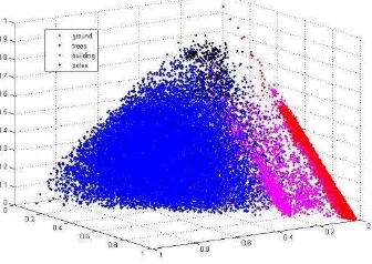
3/ 1.In this paper, trees, building, poles and ground is classified. The four kinds of objects are most common and important. The spectral features play a role in classification. In the spectral features of the points labeled into trees, the volume feature tends to be bigger than others. The surface feature of building and road is bigger. The line feature of poles is bigger. As see Figure 2, the features can be easy to distinguish the classes.
Figure 2. The spectral vectors of objects
This not only prevents over segmentation but also reduces processing time.
The result of super-voxel is showed as followed. Every color piece is a voxel. The similar feature points are grouped.
Figure 3. Super-voxel clustering
3.2 Grouping Clusters
n this stage, the clusters are grouped into segments through region growing with respect to the connectivity and normal vector of clusters. Assuming Ci has m points and Cj has n pints. The distance between Ci and Cj is defined as Equation 3.
min i j
ij k l
D p p , (3)
Where
p
ki is the position of a point in Ci,p
lj is the position of a point Cj, k1, 2 m and l1, 2 n.Then, we calculate the angle between the normal vector of a cluster and the vertical vector as Equation and the spectral similarity of clusters via the angle between two clusters as Equation 4 and 5.
arccos
,
iv i v
n
n n
, (4)
arccos , ij s si j
, (5)Where si and sj are normal vectors of Ci and Cj, respectively, and nv is the vertical vector (0, 0, 1).
The merge method is proposed by considering the connective distance
DijDth
and normal features
iv th1, ijth2
.The large-scale man-made objects can be extracted by this method. The grouping result is presented in Figure. The remaining clusters are grouped by distance.
Figure 4. Group into segments
3.3 Unary Terms
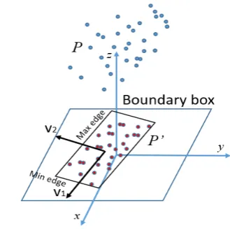
We use the output of support vector machine algorithm as unary terms. For each segment, we extract six features for training the SVM classifier. The six features are spectral vector, normal angle, height, area, edge ratio and max edge. The last three features are computed by the projective boundary box. The boundary box is obtained by the following steps:
1. Project 3d points P of a segment to the ground plane and obtain P’.
2. Compute the eigenvectors {V1, V2} of P’. The eigenvectors are the direction of boundary box edges. 3. Find the min and max value in V1 and V2 direction as
Figure 5. Then the boundary box is obtained.
Figure 5 the boundary box in ground plane
Spectral vector: the cluster geometry information.
Normal angle: The estimated normal vector of a cluster is calculated by the RANSAC method, and the angle between the estimated normal vectors.
Height: the centroid’ z value of segments. The value removes the min z which would be the height of ground plane.
Edge ratio and max edge: The edge ratio is the ratio of short edge and long edge of the projected boundary box. The ratio of pole objects would be near by 1. The ratio of building would be less than 1.
We use SVM algorithm from OpenCV. The kernel function of
SVM is Radial basis function (RBF). The iterator number is
10000.
3.4 Pairwise Terms
Pairwise terms are important to show any kind of inter-class relations. These terms are constructed as the method which is proposed by Shapovalov et al. (2010). For simplifying the model, we only obtain two neighboring features which are distance between segments and normal angle of them. Using
Bayes’ theorem, the edge probability is defined as the following equation:
1
2
1 2
1 2
| |
| ,
, i j i j i j
p f l l p f l l p l l f f
p f f
, (6)
So that, we use the edge probability as pairwise terms.
Naïve Bayes classifier is used for this problem. The two features are discreted into several grids. The distribution of the training data in the grids is the probability of the features.
3.5 Inference
Based on super-voxel, the point cloud is cut into small piece. We use the SVM to evaluate the class of every piece. Then using Naïve Bays classification, the pairwise terms are added into MRF model. We use the TRW-S algorithm to infer the final classification.
4. EXPRIMENT
4.1 Collection System
We collect point clouds data with our company mobile measurement cars as Figure 6. The car is loaded with one or two laser scanner, CCD cameras, INS (Inertia Navigation System) and GPS. The laser scanner is Rigel LiDAR. The Figure7 shows the point clouds from the Rigel LiDAR.
Figure 6. The mobile measure car
Figure 7. The point clouds from the Rigel LiDAR. The
grayscale is based on the intensity of the laser.
4.2 Result
At first, we label manually the point clouds for training the SVM model. Then check other data sets. In the experiment the above four classes have labeled.
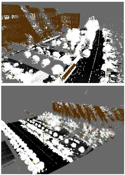
The result of the classification method is followed:
Figure 7. The classification result. The black is ground, white
Chart 1. The result of classification
ground trees poles building Recall
ground 78083 356 67 1227 0.9793
trees 1322 35368 127 7532 0.7975
poles 344 223 1342 1048 0.4538
building 2586 9442 835 24245 0.6533
precision 0.9484 0.7792 0.5660 0.7120
5. CONCLUSION
In this paper we present an approach to classify the 3d point clouds for urban area. Based on the MRF model, we use the SVM method to account for directional information. The neighborhood relations are considered into pairwise terms. It constructs an accurate model for complex scene. To overtake the insensitivity of the MRF to the large-scale objects, we use super voxel for over-segment and group the clusters into segment for large objects.
Four classes are classified in this paper. The result of the experiment shows the method is good for classification. But we must notice the classes are rough and not specific. The future work is focused on the small objects like lights and traffic signs.
REFRENCES
Munoz, D., Vandapel, N. and Hebert, M., 2008. Directional associative markov network for 3-d point cloud classification.
Shapovalov, R., Velizhev, A., Barinova, O. abd Konushin, A. , 2010. NON-ASSOCIATIVE MARKOV NETWORKS FOR POINT CLOUD CLASSIFICATION.
Aijazi, A. K., Checchin, P. and Trassoudaine, L, 2013. Segmentation based classification of 3D urban point clouds: A super-voxel based approach with evaluation. Remote Sensing, 5(4), pp. 1624-1650.
Munoz, D., Vandapel, N. and Hebert, M., 2009. Onboard contextual classification of 3-d point clouds with learned high-order markov random fields. In Robotics and Automation, 2009. ICRA'09. IEEE International Conference on. IEEE.
Daniel M., Nicolas V., Martial H., 2008. Automatic 3-D Point Cloud Classification of Urban Environments. CARNEGIE-MELLON UNIV PITTSBURGH PA.
Kolmogorov, V., 2006. Convergent tree-reweighted message passing for energy minimization. Pattern Analysis and Machine Intelligence, IEEE Transactions on, 28(10), pp. 1568-1583.
J Papon, J., Abramov, A., Schoeler, M. and Worgotter, F., 2013. Voxel cloud connectivity segmentation-supervoxels for point clouds. In Proceedings of the IEEE Conference on Computer
Vision and Pattern Recognition, pp. 2027-2034.
Zhou, Y., Yu, Y., Lu, G., and Du, S., 2012. Super-segments based classification of 3d urban street scenes. International Journal of Advanced Robotic Systems, 9.