PAN-SHARPENING APPROACHES BASED ON UNMIXING OF MULTISPECTRAL
REMOTE SENSING IMAGERY
G. Palubinskas*
Remote Sensing Technology Institute, German Aerospace Center (DLR), 82234 Wessling, Germany – [email protected]
Commission VII, WG VII/6
KEY WORDS: image processing, multi-resolution image fusion, pan-sharpening, quality assessment, model based approach, remote sensing
ABSTRACT:
Model based analysis or explicit definition/listing of all models/assumptions used in the derivation of a pan-sharpening method allows us to understand the rationale or properties of existing methods and shows a way for a proper usage or proposal/selection of new methods ‘better’ satisfying the needs of a particular application. Most existing pan-sharpening methods are based mainly on the two models/assumptions: spectral consistency for high resolution multispectral data (physical relationship between multispectral and panchromatic data in a high resolution scale) and spatial consistency for multispectral data (so-called Wald’s protocol first property or relationship between multispectral data in different resolution scales). Two methods, one based on a linear unmixing model and another one based on spatial unmixing, are described/proposed/modified which respect models assumed and thus can produce correct or physically justified fusion results. Earlier mentioned property ‘better’ should be measurable quantitatively, e.g. by means of so-called quality measures. The difficulty of a quality assessment task in multi-resolution image fusion or pan-sharpening is that a reference image is missing. Existing measures or so-called protocols are still not satisfactory because quite often the rationale or assumptions used are not valid or not fulfilled. From a model based view it follows naturally that a quality assessment measure can be defined as a combination of error model residuals using common or general models assumed in all fusion methods. Thus in this paper a comparison of the two earlier proposed/modified pan-sharpening methods is performed. Preliminary experiments based on visual analysis are carried out in the urban area of Munich city for optical remote sensing multispectral data and panchromatic imagery of the WorldView-2 satellite sensor.
* Corresponding author
1. INTRODUCTION
Multi-resolution image fusion also known as pan-sharpening aims to restore/estimate a multispectral image in a high resolution space from two given inputs: low resolution multispectral image and high resolution panchromatic image. Multi-resolution image fusion is not limited only to multispectral and panchromatic image pairs. For example, in hyper-sharpening, a high resolution image is a multispectral image, and a low resolution image is a hyperspectral image. A large number of algorithms and methods to solve this problem were introduced during the last three decades. One of the first extensive classifications of image fusion methods is presented in (Pohl and van Genderen 1998), where all methods are divided into two main groups: color related techniques, e.g. Intensity-Hue-Saturation (IHS) and statistical/numerical methods, including arithmetic combinations (addition, multiplication, difference and ratio), Principal Component Analysis (PCA), High Pass Filtering (HPF), Component Substitution (CS) and wavelets. Additionally, a combined approaches group is introduced. In (Thomas et al. 2008) the methods are grouped into three classes: projection/substitution methods (e.g. IHS, PCA); relative spectral contribution (RSC) methods, e.g. Brovey transform (BT) (Gillespie et al. 1987) and Color Normalization (CN) (Vrabel 1996); and ARSIS concept (Ranchin and Wald 2000) or its implementations, e.g.
Multi-Resolution Analysis (MRA) using wavelet transform (Aiazzi et al. 2002). Similarly as mentioned above, a hybrid methods group including all combinations of three previous groups is introduced. In (Amro et al. 2011) the methods are divided into five groups: CS family, RSC family, high-frequency injection family, methods based on the statistics of the image (e.g. Bayesian methods) and multi-resolution family (e.g. MRA). In (Xu et al. 2014) four groups are defined: CS methods (IHS, PCA, Gram–Schmidt (GS) orthogonalization), rationing methods: BT, CN, Smoothing Filter-based Intensity Modulation (SFIM) (Liu 2000), sparse representation (SR) based methods (Li and Yang 2011, Zhu and Bamler 2013, Vicinanza et al. 2015) and ARSIS concept or MRA methods. In (Yang and Zhang 2014) it is shown that three groups of methods based on component substitution, modulation and multi-resolution analysis can be expressed using a generalized model. In recent review (Pohl and van Genderen 2015), which is an update of the old review (Pohl and van Genderen 1998), methods are divided into five groups: CS, numerical and statistical image fusion, modulation-based techniques, multi-resolution approaches and hybrid techniques. In (Zhang and Huang 2015) a new look at image fusion methods from a Bayesian perspective is presented, which shows that CS and MRA based methods are special cases of Bayesian based method under Gaussian model assumption.
i
In summary, the most known and popular methods can be divided into two large groups (Vivone et al. 2015, Palubinskas 2015). The first group of methods is based on a linear spectral transformation, e.g. IHS, PCA, and GS, followed by a CS. Methods of the second group use spatial frequency decomposition usually performed by means of High Pass Filtering, e.g. boxcar filter (HPF) in signal domain, filtering in Fourier domain or MRA using wavelet transform. Additionally, we would like to mention presently quite a small group of methods, but which are spreading quite rapidly in remote sensing community. These are so-called model based methods based on the minimization of model error residuals, e.g. using Bayesian (Aanæs et al. 2008, Fasbender et al. 2008, Zhang et al. 2012, Aly and Sharma 2014, Palsson et al. 2014, Loncan et al. 2015) or already mentioned SR based techniques. One of the main reasons, why it is so difficult to classify existing methods is a missing common denominator. We propose to use models/assumptions, which are used in a method derivation, as a basis for different method comparison. First attempts of such type classification were already performed, e.g. using image formation model (Wang et al. 2005). Thus, we propose to look at image fusion methods from a model based view. This type of analysis allows us to recognize quite easily similarities and differences of various methods and thus perform a systematic classification of most known multi-resolution image fusion approaches and methods.
In parallel to the development of pan-sharpening methods, many attempts were undertaken to assess quantitatively their quality usually using measures originating from signal/image processing. Examples of measures (scalar or vector based) used to assess pan-sharpening quality are Spectral Angle Mapper (SAM), Mean Squared Error (MSE) and measures based on it, e.g., Peak Signal-to-Noise Ratio (PSNR), Relative Average Spectral Error (RASE) and relative dimensionless global error in synthesis (ERGAS), Pearson’s Correlation Coefficient (CC), Universal Image Quality Indices (UIQI/SSIM) and multispectral extensions of UIQI (Q4/Q2n) just to mention few or most popular of them. For recent overviews of quality measures, see references (Alparone et al. 2007, Ehlers et al. 2010, Aiazzi et al. 2011, Makarau et al. 2012, Palubinskas 2015). These simple/separate measures can be used only as Full Reference (FR) measures that is, when the reference image is available. This situation is valid for quite few applications mostly simulations. Due to the missing reference in pan-sharpening quality assessment task different solutions or so-called protocols were proposed: Wald’s protocol (Wald et al. 1997), Zhou’s protocol (Zhou et al. 1998), Quality with No Reference (QNR) (Alparone et al. 2008) and Khan’s protocol (Khan et al. 2009), which usually include the calculation of several quality measures. Of course, a sole or joint quality measure, as already proposed in (Alparone et al. 2008, Padwick et al. 2010, Palubinskas 2015), enables much easier and practical/comfortable ranking of various fusion methods.
But besides that, most of existing quality measures cannot satisfy fully the needs of remote sensing community for different methods evaluation or comparison. Again, we propose to look at quality assessment problem from a model based perspective. Thus, we propose to select common models used by most of fusion methods and to define a quality measure by combining such model error residuals.
This paper presents a new view to pan-sharpening task – model based view – in the following section (Sect. 2). This analysis allows us to understand the origin or rationale of most known
methods and additionally results in a proposal of new methods or shows a way for the modification of existing methods. Moreover, this analysis resulted in the proposal of new quality measures or a way how to construct new measures which have a potential for a future. Finally, the paper ends with conclusion and reference sections.
2. METHODOLOGY
A model based view at pan-sharpening or multi-resolution image fusion and its quality assessment is presented. This analysis allowed us to show the origin and drawbacks of most popular methods and a proposal or selection of methods which really respect models assumed.
2.1 Aim
The aim is to restore/estimate a multispectral image msf in the resolution of panchromatic image pan, from low resolution multispectral image ms using a high resolution panchromatic image pan. It is known as a pan-sharpening or multi-resolution image fusion task. To solve this task various assumptions or models can or should be made. Quite often not all assumptions are explicitly written. Further in this paper the assumptions or models assumed are underlined. Notations used in this paper are given in Tables 1-3.
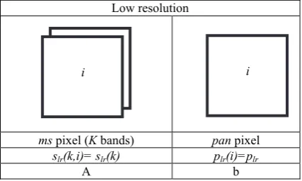
Low resolution
ms pixel (K bands) pan pixel
slr(k,i)= slr(k) plr(i)=plr
A b
Table 1. Definition and notation of input, intermediate and output pixels of pan-sharpening: (a) multispectral pixel with K
spectral bands (index i is used), (b) panchromatic pixel in low resolution (index i is used).
High resolution
msi pixel (interpolation) msf pixel (fusion)
slr(k,j) shr(k,j)
a b
Table 2. Definition and notation of input, intermediate and output pixels of pan-sharpening: (a) interpolated multispectral
pixel to the resolution of pan, (b) result of pan-sharpening (index j is used for high resolution pixels in the area occupied
by ms pixel i).
i
j j
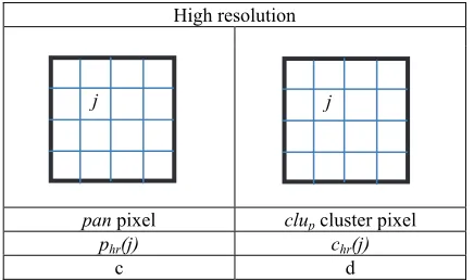
High resolution
pan pixel clup cluster pixel
phr(j) chr(j)
c d
Table 3. Definition and notation of input, intermediate and output pixels of pan-sharpening: (a) panchromatic pixel in high resolution, (b) cluster pixel of pan (index j is used for high
resolution pixels in the area occupied by ms pixel i).
Index ni is used to denote pixels in some neighborhood/window
(e.g. 3x3 pixels as used later in this paper) of pixel i in ms image. A box with a bold line shows image area occupied by ms pixel i
in pan image (index j is used to denote pixels in a high resolution image) (see Table 2. or 3). Again, index nj is used to denote pixels
in some neighborhood/window of pixel j in pan image, e.g. used for filtering in HPFM and MRA methods. Bold symbols are used for vectors and matrices.
2.2 General models/assumptions
The following three implicit assumptions are valid for pan-sharpening. First, the spatial resolution of ms is lower than the resolution of pan. Second, ms exhibits more spectral bands than
pan. Third, spectra of both data overlap significantly.
For each ms pixel i (index i is omitted for simplicity further) the following four assumptions (1-4) can be formulated, which are based on a common sense of image formation/acquisition model.
Spectral consistency for low resolution multispectral data (Model 1)
lr k
lr k p
s k
w
( ) ( ) (1)where w(k) are spectral weights calculated from spectral response functions of data provider (Boggione et al. 2003) and sum to
( )1k
k
w . This assumption gives a relation between
the input of pan-sharpening task: a low resolution multispectral image slr and an unknown panchromatic band in a low
resolution plr . We will show later that it appears to be useful in
derivation of image fusion methods and thus is used further for an approximation or estimation of plr.
Spectral consistency for high resolution multispectral data (Model 2)
i j j p j k s k
w hr
k
hr
( ) ( , ) ( ) (2)This assumption gives a relation between input phr and output
shr of pan-sharpening task, thus is essential further.
Spatial consistency for multispectral data (Model 3)
k k s j k s j k
f lr
j
hr
s
( , ) ( , ) ( ) (3)where fs are low pass filters with f k j k
j
s
( , ) 1 . Again, this assumption gives a relation between input slr and output shrof pan-sharpening task, thus is essential further.
Spatial consistency for panchromatic data (Model 4)
lr j
hr p j p j p
f
( ) ( ) (4)wherefpis a low pass filter with
( )1j p j
f . This assumption
gives a relation between the input of pan-sharpening task phr
and an unknown panchromatic band in a low resolution plr . We
will show later that it appears to be useful in derivation of image fusion methods and thus is used further as an alternative to (1) for an approximation or estimation of plr.
For each model or assumption an error term should be added, which is omitted for simplicity.
If we assume that both assumptions (1,4) are valid simultaneously, then it appears that both filters fs and fp should
be equal (see Appendix 1). But, this is not always valid in real applications. So simultaneous usage of assumptions (1,4) imply too strong restrictions and thus are not very useful in praxis. Usually only one these two assumptions is used, depending on the way how plr is calculated/estimated.
Thus only the following two assumption combinations: (1,2,3) or (2,3,4) are used further in this paper.
Additionally, the following noise observation model (Model 5) is assumed
n n t
o , ~N(0,) (5)
where o – observation sample, t – true signal, n - additive noise with a standard deviation . o can be, e.g. s (spectral image) or
p (panchromatic image) in this context. For example, (5) can be written as slr(k)shr(k)n in some homogeneous image area.
It can be seen that assumptions (1-5) depend on parameters w,
fs, fp and , which may be given or have to be estimated from
data. For example, w can be estimated using (4) and (1), when fp is known.
Additional assumptions may concern the accuracy of the absolute/relative radiometric calibration of ms and pan data, and the spatial co-registration of ms and pan data (Baronti et al. 2011).
2.3 Pan-sharpening methods
In the pan-sharpening task usually the following two general models (2) and (3) are assumed. Moreover, implicitly the model (1) or (4) and the model (5) are assumed.
For example, for WorldView-2 satellite remote sensing data assumption (2) results in 4x4=16 equations and assumption (3) in 8 equations. So in total 24 equations are available to estimate in total 16*8=128 unknowns. Thus, a pan-sharpening task is an ill-posed problem.
j j
To solve it additional assumptions or more specific models are needed. Here, we will show how a pure pixels assumption leads to an analytic solution of pan-sharpening task. Its relation to several known image fusion methods is presented. Further, the two methods are presented for pan-sharpening of mixed pixels, which respect models assumed. Finally, other so-called model based methods minimizing model error residuals are shortly introduced.
2.3.1 Pure pixels assumption: A pure pixels assumption (Model 6), which is usually defined for some homogeneous image area, implies the following relationship for each k
i
This assumption reduces a pan-sharpening task to the estimation of only 8 unknowns and thus allows an analytic solution of the problem. From (6) and (2) it follows directly
i
Under the pure pixels assumption from (2) follows
hr
derivation of (10).
Thus, from (10) we have a solution of a pan-sharpening task
k k s k
shr( ) lr( ) (11)
with the condition (9) to be fulfilled. This is a trivial, but very important solution of the problem because it is analytic. We have to note, that under the assumption (1) the condition (9) reduces to
hr lr p
p (12)
In praxis, quite often equation (12) does not hold, e.g. due imperfect/missing absolute data calibration. Thus, the following two assumptions: multiplicative constant shift in panchromatic band (Model 13)
or additive constant shift in panchromatic band (Model 14) can be assumed
Then from (12) and (13) the solution (11) can be written for multiplicative model as
)
and from (12,14) for additive model
lr
Due to the assumption (5) for panchromatic image the definition of pure pixels (8) can be relaxed to
) (Phr
stddev (17)
In this case, from (15) follows directly
)
Equations (18,19) present analytic solutions of the pan-sharpening task under the assumptions (1,2,3,5,17) or simply for pure pixels for additive (13) and multiplicative (14) models respectively. We have to note that this solution accounts for the variation of pixel values in high resolution panchromatic image, what it makes different from a trivial solution (11). This solution is valid only for pure pixels (17).
2.3.2 Connection to the known image fusion methods: Here we will show exemplary, how several well-known methods, e.g. Intensity Hue Saturation (IHS) transformation, Color Normalization (CN), Smoothing Filter-based Intensity Modulation (SFIM), High Pass Filtering Method (HPFM) or Multi-resolution Analysis (MRA) methods are related to (18) or (19).
Though (18) is derived for a pure pixels assumption, it can be easily modified in order to be applied to all pixels including mixed pixels too (violation of pure pixels assumption!) in the following way (sometimes called modulation)
)
Similarly (19) can be modified
)
WorldView-2 data, e.g. 4x4 pixels). In summary, a list of several known methods which can be derived directly from (18, 19) is presented in Table 4.
Parameters
Table 4. A list of pan-sharpening methods derived from (18, 19).
Here we have to note that additionally to the already mentioned drawback (violation of pure pixels assumption), these methods use interpolation of ms to msi, what includes wrong (non-existent) information into the fusion result for heterogeneous image areas.
So we see that all these well-known methods are based on the same assumptions or models as (18) or (19) and thus they can be considered model based methods. It is not so easy to see that
because quite often the assumptions used are not defined explicitly. For example, attempts of such analysis based on image formation principle can be seen already in (Liu 2000, Wang et al. 2005, Aanæs et al. 2008), though not all models used are written explicitly. So the methods (18,19) can be seen as an optimal pan-sharpening methods for pure pixels. Application of these methods for mixed pixels, as its derivatives such as IHS/CN/SFIM/HPF/HPFM/MRA do, can lead to wrong/incorrect fusion results because the pure pixels assumption is violated. This is maybe the main reason, why most of the fusion methods developed in last decades cannot satisfy fully the remote sensing community, maybe except the visual perception task.
Here we have to note that the assumptions (13,14) can be fulfilled by appropriate histogram matching of data or absolute calibration of input data used in pan-sharpening task.
2.3.3 Mixed pixels: In heterogeneous image areas pure pixels are quite seldom and the most pixels are mixed that is composed of several components or so-called endmembers (or pure spectra). From (8) and (17) it follows that mixed pixels satisfy the following condition: stddev(Phr) . These mixed pixels should be unmixed before the fusion can be performed. Two different approaches are presented below, which respect models assumed.
2.3.3.1 Linear mixing model. A very popular approach to unmix mixed pixels is to assume a linear mixing model (Settle and Drake 1993) abundances of endmembers (unknowns) and e – error residuals. The solution of (24) can be found, e.g. by a Bounded-Variable Least-Squares (BVLS) minimization (Stark and Parker 1995) of the following error residual or norm
2
This spectral unmixing model assumes the knowledge of endmembers a priori (e.g. from spectral library, ms data clustering, pure pixels model or the usage of any other spectral tool to extract em) and estimates abundances α of each em within the ms pixel. The number of endmembers M is limited by the number of spectral bands K or equations in (24). Usually the number of em for a single ms pixel reduces to M’<M due to zero valued abundances. Thus, recently proposed methods based on the compressed sensing theory and sparse representation (Candès and Wakin 2008) can be preferable than BVLS.
Pan-sharpening based on endmembers can be performed following the way proposed in (Bieniarz et al. 2011, 2014) and (Yokoya et al. 2012) for hyperspectral and multispectral image fusion (hyper-sharpening) with some modifications, which are
specific for a pan-sharpening task. First, an unmixing of ms
pixel is performed by using estimated/given multispectral endmembers em (25). Then, non-zero em are resampled spectrally to endmembers of pan (2)
Further steps are specific for a pan-sharpening task. Third, pan
pixels covering ms pixel i are clustered into several clusters, e.g. a number of clusters is a number of endmembers M’ in ms
pixel. For example, k-means or multi-mode histogram thresholding can be used. The clustering method should account for the size of clusters given by (m). Fourth, pixels belonging to one cluster, e.g. c are related to emp by using the following minimization
where mean(.) is a mean value of pan values belonging to cluster c. Similarly as in (13)
possible shift between phr and emp should be corrected
energy preservation assumption in one ms pixel). Finally, msf is calculated for each cluster c ask
A local approach, that is the usage of individual ms pixel or its neighbourhood/window, is preferable twofold. First, it is used to avoid ambiguity in (29) due to many-to-one relationship between ms and pan data(2). Second, it allows us to increase the number of equations in (24) in order to match the limited number of bands K. Careful selection of a window size is important. On one hand, the window size should be large enough to include all endmembers present in ms pixel. On the other hand, it should be not too large in order to limit the number of endmembers to K. Already available/detected pure pixels can be used as endmembers.
2.3.3.2 Spatial unmixing (or unmixing-based data fusion).
Another possible approach to perform image fusion is to perform the interchange unknown variables in (24), that is to estimate endmembers from the known abundances as it is proposed in (Zhukov et al. 1999, Clevers and Zurita-Milla 2008). First, the abundances for each ms pixel i can be estimated from the pan image clustering clup (see Table 1), e.g. M clusters. Then, the spatial unmixing is used to estimate endmembers in ms pixel i separately for each k
where the number of equations in (30) is given by the selected neighborhood, e.g. 3x3 of ms pixel i. Here, the same minimization methods (e.g. BVLS) can be used as in the previous section 2.3.3.1 to solve equation system (30). High resolution msf image is then reconstructed using estimated em values
The size of the neighborhood (number of pixels) or number of equations (30) should be larger than M.
There are still some open issues concerning the usage of pure pixels information in spatial ummixing, the usage of already available pure pixels information in the reconstruction method of shr , selection of a number of clusters M in pan image and the
size of the neighborhood of ms pixel i . Finally, the future research could be directed towards the comparison of both image fusion methods.
2.3.4 Minimization of model error residuals: Model based methods are formulated usually as optimization problems which minimize some cost functions based on image formation/observation models. Most of the methods are based on the following two general assumptions or models (2,3). Thus, in general a minimization of a sum of error residuals of these two models with some regularization function imposed on the solution is used, e.g. as
2 3 ( )
regularization parameters, F – some regularization function. Usually these error residuals are written in a form of matrices (Li and Yang 2011). Most of these fusion methods differ mainly in F definition, e.g. F is a total variation in (Palsson et al. 2014), ERM3 is applied only on high frequency components of signal and F is a spectral correlation dependent regularization (Aly and Sharma 2015). Moreover, the methods can be formulated using a Bayesian (Fasbender et al. 2008, Zhang et al. 2012, Zhang and Huang 2015) or sparsity regularization frameworks (Li and Yang 2011, Zhu and Bamler 2013, Vicinanza et al. 2015). Further, unmixing models can be included into the cost function definition as, e.g. in (Yokoya et al. 2012, Loncan et al. 2015).2.4 Pan-sharpening quality assessment
A natural way to estimate the quality of pan-sharpening in the absence of a reference is to use model error residuals. As it is shown in the previous section most of fusion methods use/assume the models (2,3). Thus, these models can be used as a common denominator to compare or assess the quality of image fusion methods as already proposed in (Palubinskas 2015).
From Model (2) we have a Quality measure in High Resolution (QHR)
Composite measure based on Means, Standard deviations and Correlation (CMSC) is defined (Palubinskas 2014) as
signal/image patches x, y; ρ is Pearson’s correlation coefficient and R = 28− 1 = 255 for 8bit data.From Model (3) we have a Quality measure in Low Resolution (QLR)
filter, which is band dependent, —convolution operator, means decimating of high resolution data to a low resolution scale.
One more model that is Model (5) is assumed implicitly practically in all fusion methods. Thus, it can be used to define an additional quality measure: Quality measure based on Noise (QN), which can be based on the comparison of noise values (standard deviations) in homogeneous areas of images slr and shr
2These three separate quality measures can be used to produce a joint quality measure as, e.g. in (Palubinskas 2015)
1
Additionally, method specific assumptions or models (error residuals) can be used to characterize the behavior of a particular method sometimes called a quality layer. For example, from pure pixels assumption (8,17) we can define a measure for pure pixels
) (
1 stddev Phr
QPP (39)
Similarly, for mixed pixels we can use model error residuals as quality measures.
3. PRELIMINARY EXPERIMENTS
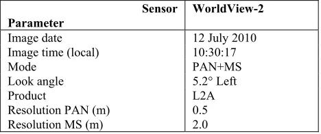
I will illustrate my ideas concerning pan-sharpening quality assessment for optical remote sensing satellite WorldView-2 (WV-2) data over Munich city in Germany. For scene details see Table 5.
Sensor Parameter
WorldView-2
Image date 12 July 2010
Image time (local) 10:30:17
Mode PAN+MS
Look angle 5.2° Left
Product L2A Resolution PAN (m) 0.5
Resolution MS (m) 2.0
Table 5. Scene parameters for WorldView-2 data over the city of Munich, Germany.
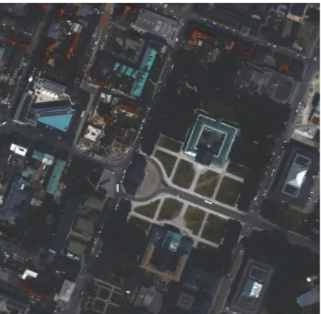
Original data are presented in Figure 1 (panchromatic band) and Figure 2 (bilinear interpolated multispectral RGB bands). Pure pixels derived using (17) are shown in Figure 3 and they occupy about 15% of the whole scene. The result of
reconstruction of only pure pixels using an optimal pan-sharpening method (19) is presented in Figure 4. Further, results of reconstruction using the two methods (29) and (31) based on linear unmixing are presented in Figures 5 and 6 respectively. For the visual quality evaluation the result of HPFM (Palubinskas 2013) is included in Figure 7. We see, that unmixing based methods are competitive with known methods and thus have a potential for applications such as classification and change detection. Optimization of the methods and quantitative analysis is still to be performed using new quality measures.
Figure 1. Panchromatic band of WV-2 scene.
Figure 2. Bilinear interpolated bands: 5, 3, 2 of WV-2 scene.
Figure 3. Pure pixels detected in WV-2 scene (about 15%).
Figure 4. Reconstruction of pure pixels using (19).
Figure 5. Reconstruction using spectral unmixing model (29).
Figure 6. Reconstruction using spatial unmixing (31).
4. CONCLUSIONS
Model based analysis of most existing pan-sharpening methods showed that they are based mainly on the two models or assumptions: spectral consistency for high resolution multispectral data and spatial consistency for multispectral data. Additionally, spectral transformation and filtering based methods are based on a pure pixels assumption. Thus, their usage for mixed pixels can lead to wrong image fusion results. Two methods, one based on a linear unmixing model and another one based on a spatial unmixing, are described which respect models assumed and thus can produce correct or physically justified fusion results. Model based methods based on Bayesian and sparse representation frameworks are still in the development, but seem to be very promising.
Figure 7. Reconstruction using HPFM (Palubinskas 2013).
From the model based analysis it followed that error residuals of general or common models can be used as quality assessment measures of multi-resolution image fusion methods in the absence of a reference image. These models include the following general or common assumptions: spectral consistency for high resolution multispectral data, spatial consistency for multispectral data and additive noise observation model. They can be combined to define a sole or joint quality measure for a more convenient/comfortable quality measure.
Presented analysis is not limited only to the pan-sharpening. It can be easily extended to the hyper-sharpening too.
The future work could be directed towards a model based classification of all multi-resolution image fusion methods, a comparison of the two proposed/modified pan-sharpening methods with already existing model based methods using proposed quality assessment measures.
ACKNOWLEDGEMENTS
I would like to thank DigitalGlobe and European Space Imaging (EUSI) for the collection and provision of WorldView-2 scene over the Munich city.
REFERENCES
Aanæs, H., Sveinsson, J.R., Nielsen, A.A., Bøvith, T., and Benediktsson, J.A., 2008. Model-based satellite image fusion.
IEEE Transactions on Geoscience and Remote Sensing, 46 (5),
1336-1346.
Aiazzi, B., Alparone, L., Baronti, S., and Garzelli, A., 2002. Context-Driven Fusion of High Spatial and Spectral Resolution Images Based on Oversampled Multiresolution Analysis. IEEE
Transactions on Geoscience and Remote Sensing, 40 (10),
2300-2312.
Alparone, L., Wald, L., Chanussot, J., Thomas, C., Gamba, P., and Bruce, L.M., 2007. Comparison of pansharpening algorithms: Outcome of the 2006 GRS-S data-fusion contest.
IEEE Transactions on Geoscience and Remote Sensing, 45
(10), 3012-3021.
Alparone, L., Aiazzi, B., Baronti, S., Garzelli, A., Nencini, F., and Selva, M., 2008. Multispectral and panchromatic data fusion assessment without reference. Photogramm. Eng. Remote Sens. 74 (2), 193–200.
Aly, H.A., and Sharma, G., 2014. A Regularized model-based optimization framework for pan-sharpening. IEEE Transactions on Image Processing, 23 (6), 2596-2608.
Amro, I., Mateos, J., Vega, M., Molina, R., and Katsaggelos, A., 2011. A survey of classical methods and new trends in pansharpening of multispectral images. EURASIP J. Adv. Signal Process., 2011, 79, 1–22.
Baronti, S., Aiazzi, B., Selva, M., Garzelli, A., and Alparone, L., 2011. A theoretical analysis of the effects of aliasing and misregistration on pansharpened imagery. IEEE Journal of Selected Topics In Signal Processing 5 (3), 446-453.
Bieniarz, J., Cerra, D., Avbelj, J., Müller, R., and Reinartz, P., 2011. Hyperspectral image resolution enhancement based on spectral unmixing and information fusion. In: International Archives of the Photogrammetry, Remote Sensing and Spatial
Information Sciences, ISPRS Hannover Workshop, 14-17 June
2011, Hannover, Germany, Vol. XXXVIII-4/W19, 33-36.
Bieniarz, J., Müller, R., Zhu, X.X., and Reinartz, P., 2014. Hyperspectral image resolution enhancement based on joint sparsity spectral unmixing. In: Proc. IGARSS, 13-18 July, Quebec City, QC. Piscataway, NJ: IEEE, 2645-2648.
Boggione, G.A., Pires, E.G., Santos, P.A., and Fonseca, L.M.G., 2003. Simulation of panchromatic band by spectral combination of multispectral ETM+ bands. In: Proceedings of International Symposium on Remote Sensing of Environment
ISRSE, 10-44 November, Honolulu, HI. Tucson, AZ: ICRSE,
1-3.
Candès, E.J., and Wakin, M.B., 2008. An introduction to compressive sampling. IEEE Signal Processing Magazine, 25 (2), 21-30.
Chavez, P.S., Sides, S.C., and Anderson, J.A., 1991. Comparison of three different methods to merge multiresolution and multispectral data: Landsat TM and SPOT panchromatic.
Photogrammetric Engineering & Remote Sensing, 57 (3), 295– 303.
Clevers, J.G.P.W., and Zurita-Milla, R., 2008. Multisensor and multiresolution image fusion using the linear mixing model. In: T. Stathaki, ed. Image Fusion: Algorithms and Applications. London, UK:Academic Press, 67-84.
Ehlers , M., Klonus, S., Åstrand, P.J., and Rosso, P., 2010. Multisensor image fusion for pansharpening in remote sensing,
International Journal of Image and Data Fusion 1 (1), 25-45.
Fasbender, D., Radoux, J., and Bogaert, P., 2008. Bayesian data fusion for adaptable image pansharpening. IEEE Transactions
on Geoscience and Remote Sensing, 46 (6), 1847-1857.
Gillespie, A.R., Kahle, A.B., and Walker, R.E., 1987. Color enhancement of highly correlated images—II Channel ratio and ‘chromacity’ transformation techniques. Remote Sens. Environ., 22 (3), 343–365.
Khan, M.M., Alparone, L., and Chanussot, J., 2009. Pansharpening quality assessment using the modulation transfer functions of instruments. IEEE Trans. Geosci. Remote Sens. 47 (11), 3800–3891.
Li, S., and Yang, B., 2011. A new pan-sharpening method using a compressed sensing technique. IEEE Trans. Geosci. Remote Sens. 49 (2), 738–746.
Liu, J.G., 2000. Smoothing-based intensity modulation: a spectral preserve image fusion technique for improving spatial details. International Journal of Remote Sensing, 21 (18), 3461-3472.
Loncan, L., Almeida, L.B., Bioucas-Dias, J.M., Briottet, X., Chanussot, J., Dobigeon, N., Fabre, S., Liao, W., Licciardi, G.A., Simoes, M., Tourneret, J.-Y., Veganzones, M.A., Vivone, G., Wei, Q., and Yokoya, N., 2015. Hyperspectral pansharpening: a review. IEEE Geoscience and Remote Sensing Magazine, 3 (3), 27-46.
Makarau, A., Palubinskas, G., and Reinartz, P., 2012. Analysis and selection of pan-sharpening assessment measures. Journal of Applied Remote Sensing, 6 (1), 063548, 1-20.
Padwick, C., Deskevich, M., Pacifici, F., and Smallwood, S., 2010. WorldView-2 pan-sharpening. In: Proceedings of ASPRS, 26-30 April, 2010, San Diego, USA, Bethesda, MD:ASPRS.
Palubinskas, G., and Reinartz, P., 2011. Multi-resolution, multi-sensor image fusion: general fusion framework. In: U. Stilla, P. Gamba, C. Juergens, and D. Maktav, eds. Proc. of Joint Urban
Remote Sensing Event (JURSE), 30 March-1 April, Munich,
Germany. Piscataway, NJ: IEEE.
Palubinskas, G., 2013. Fast, simple and good pan-sharpening method. Journal of Applied Remote Sensing, 7 (1), 073526, 1-12.
Palubinskas, G., 2014. Mystery behind similarity measures MSE and SSIM. In: Proc. International Conference on Image
Processing (ICIP), 27-30 October, 2014, Paris, France.
Piscataway, NJ: IEEE, 575-579.
Palubinskas, G., 2015. Joint quality measure for evaluation of pansharpening accuracy. Remote Sensing, 7 (7), 9292-9310.
Palsson, F., Sveinsson, J.R., and Ulfarsson, M.O., 2014. A new pansharpening algorithm based on total variation. IEEE Geoscience and Remote Sensing Letters, 11 (1), 318-322.
Pohl, C., and van Genderen, J., 1998. Review article Multisensor image fusion in remote sensing: concepts, methods and applications. International Journal of Remote Sensing, 19 (5), 823–854.
Pohl, C., and van Genderen, J., 2015. Structuring contemporary remote sensing image fusion. International Journal of Image and Data Fusion, 6 (1), 3–21.
Ranchin, T., and Wald, L., 2000. Fusion of high spatial and spectral resolution images: The ARSIS concept and its implementation. Photogramm. Eng.Remote Sens. 66 (1), 4–18.
Settle, J.J., and Drake, N.A., 1993. Linear mixing and the estimation of ground cover proportions. International Journal of Remote Sensing, 14 (6), 1159-1177.
Stark, P.B., and Parker, R.L., 1995. Bounded-variable least-squares: an algorithm and applications. Computational Statistics, 10, 129-141.
Thomas, C., Ranchin, T., Wald, L., and Chanussot, J., 2008. Synthesis of multispectral images to high spatial resolution: a critical review of fusion methods based on remote sensing physics. IEEE Transactions on Geoscience and Remote Sensing, 46 (5), 1301–1312.
Tu, T.-M., Su, S.-C., Shyu, H.-C., and Huang, P.S., 2001. A new look at IHS-like image fusion methods. Information Fusion, 2 (3), 177–186.
Vicinanza, M.R., Restaino, R., Vivone, G., Dalla Mura, M., and Chanussot, J., 2015. A pansharpening method based on the sparse representation of injected details. IEEE Geoscience and Remote Sensing Letters, 12 (1), 180-184.
Vivone, G., Alparone, L., Chanussot, J., Dalla Mura, M., Garzelli, A., Licciardi, G.A., Restaino, R., and Wald, L., 2015. A critical comparison among pansharpening algorithms. IEEE
Transactions on Geoscience and Remote Sensing, 53 (5),
2565-2586.
Vrabel, J., 1996. Multispectral imagery band sharpening study.
Photogrammetric Engineering & Remote Sensing, 62 (9), 1075– 1083.
Wald, L., Ranchin, T., and Mangolini, M., 1997. Fusion of satellite images of different spatial resolutions: Assessing the quality of resulting images. Photogramm. Eng. Remote Sens. 63 (6), 691–699.
Wang, Z., Ziou, D., Armenakis, C., Li, D., and Li, Q., 2005. A comparative analysis of image fusion methods. IEEE
Transactions on Geoscience and Remote Sensing, 43 (6),
1391-1402.
Xu, Q., Zhang, Y., and Li, B., 2014. Recent advances in pansharpening and key problems in applications. International Journal of Image and Data Fusion, 5 (3), 175–195.
Yang, J., and Zhang, J., 2014. Pansharpening: from a generalised model perspective. International Journal of Image and Data Fusion, 5 (4), 285–299.
Yokoya, N., Yairi, T., and, Iwasaki, A., 2012. Coupled nonnegative matrix factorization unmixing for hyperspectral and multispectral data fusion. IEEE Transactions on
Geoscience and Remote Sensing, 50 (2), 528-537.
Zhang, L., Shen, H., Gong, W., and Zhang, H., 2012. Adjustable model-based fusion method for multispectral and panchromatic Images. IEEE Transactions on Systems, Man, and
Cybernetics—Part b: Cybernetics, 42 (6), 1693-1704.
Zhang, H.K., and Huang, B., 2015. A new look at image fusion methods from a Bayesian perspective. Remote Sensing 7 (6), 6828-6861.
Zhou, J., Civco, D.L., and Silander, J.A., 1998. A wavelet transform method to merge Landsat TM and SPOT panchromatic data. Int. J. Remote Sens. 19 (4), 743–757.
Zhu, X.X., and Bamler, R., 2013. A sparse image fusion algorithm with application to pan-sharpening. IEEE
Transactions on Geoscience and Remote Sensing, 51 (5),
2827-2836.
Zhukov, B., Oertel, D., Lanzl, F., and Reinhäckel, G., 1999. Unmixing-based multisensor multiresolution image fusion.
IEEE Transactions on Geoscience and Remote Sensing, 37 (3),
1212-1226.
APPENDIX
Equality of low pass filters under simultaneous validity of assumptions (1,4)
If we assume that both assumptions (1,4) are valid simultaneously
k
lr j
hr
p j p j wk s k
f ( ) ( ) ( ) ( ) (A.1)
then from (2) and (A.1) it follows
k k s j k s j
f lr
j
hr
p
( ) ( , ) ( ) (A.2)Thus from (A.2) and (3) it should be
k j f j k
fs( , ) p( ) (A.3)