RESOLUTION IN PHOTOVOLTAIC POTENTIAL COMPUTATION
N. Alam a, 1*, V. Coors a, S. Zlatanova b, P. J. M. Oosterom b
a
Faculty of Surveying, Computer Science and Mathematics, Stuttgart University of Applied Sciences, Schellingstr. 24, 70174 Stuttgart, Germany - (nazmul.alam, Volker.coors)@hft-stuttgart.de
b
OTB, GIS-technology, Delft University of Technology, Jaffalaan 9, 2628 BX Delft, The Netherlands – (S.Zlatanova, P.J.M.vanOosterom)@tudelft.nl
KEY WORDS: Solar Potential, Shadow, Meshing Resolution, Time Interval, Sky View Factor, CityGML
ABSTRACT:
In this paper, an analysis of the effect of the various types of resolution involved in photovoltaic potential computation is presented. To calculate solar energy incident on a surface, shadow from surrounding buildings has been considered. The incident energy on a surface has been calculated taking the orientation, tilt and position into consideration. Different sky visibility map has been created for direct and diffuse radiation and only the effect of resolution of the factors has been explored here. The following four resolutions are considered: 1. temporal resolution (1, 10, 60 minutes time interval for calculating visibility of sun), 2. object surface resolution (0.01, 0.1, 0.375, 0.75, 1.25, 2.5 and 5 m2 as maximum triangle size of a surface to be considered), 3. blocking obstacle resolution (number of triangles from LoD1, LoD2, or LoD3 CityGML building models), and 4. sky resolution (ranging from 150 to 600 sky-patches used to divide the sky-dome). Higher resolutions result in general in more precise estimation of the photovoltaic potential, but also the computation time is increasing, especially as realizes that this computation has to be done for every building with its object surface (both roofs and façades). This paper is the first in depth analysis ever of the effect of resolution and will help to configure the proper settings for effective photovoltaic potential computations
* Corresponding author.
1. INTRODUCTION
Urbanization leads to a very high increase of energy use. Buildings are the largest consumers of energy in cities. For large scale implementation in the urban areas building integrated photovoltaic system is an appropriate option. So it is essential to develop the appropriate tools and methods for solar potential analysis. Most of the traditional methods focus only on the roof surface but modern cities contain lot of other potential area like on vertical façades for photovoltaic installation other than roof surface.
Generally, energy production from photovoltaic system depends of incident solar energy and photovoltaic efficiency. Efficiency of photovoltaic cell depends on spectrum and intensity of incident light and temperature of the cell. Solar energy incident upon a surface depends on longitude, latitude, sun angles, surface tilt, surface orientation, contribution of direct and diffuse radiation, absorption, reflectance, shadow caused by surrounding objects such as buildings and vegetation. To be able to simulate all these factors and provide good estimates of best roof and façade surface for photovoltaic cells, three types of resolutions are investigated: the resolution of 3D city models, the time interval used for the computations and the resolution of the sky. Two types of 3D model resolution can be distinguished: a surface resolution (i.e. max triangle size used to represent each surface) and a blocking obstacle resolution (number of triangles while using different LODs). Estimations of photovoltaic potential can be prepared for different intervals, e.g. minutes, hours, days, months or a year, and a different sky resolution (i.e. number of patches a sky can be subdivided). The higher the resolution, the better representation of the real-world situation. However, high models computational expensive. Therefore it is critical to investigate the effect of the different resolutions on the accuracy of the photovoltaic computations.
The main research interest in this study was twofold: 1) to determine the added value of including shadow consideration in the simulation models and 2) to devise a fast shadow detection method. The study considered roofs and façades. It investigated what the minimal needed resolution is to be able to obtain reliable estimates. This paper presents the methodology for the computation and analysis of photovoltaic potential of a region for BIPV (Building Integrated Photovoltaic) module. For the tests available 3D city models of German cities were used as case study area like Scharnhauser Park, Grünbühl, Ludwigsburg and some custom test models.
The paper is organised as follows. The state of the art of solar potential followed by description of the solar radiation parameters of interest is presented first. Then the methodology has been explained very briefly and separately at each part. Then the Sky View Factor has been highlighted and its role in this research has been explained. After that the factors like incorporating both terrain and near surface shadowing using GRASS and r.sun module. They compared the trade-off of each computation option: spatial resolution, time step and shading effect. Tooke et al. have showed the seasonal influences of tree on solar potential for rooftop panels using LiDAR (light detection and ranging) (National Ocean Service, 2015) data. Freitas et al (Freitas, et al., 2015) have done a detailed state-of-the-art review of the models ranging from simple 2D
visualization and solar constant methods, to more sophisticated 3D representation and analysis. Ramírez-Faz et al. (Ramírez-Faz, et al., 2015) presented a general mathematical method to obtain projection equation in vertical plane using Sky View Factor (SVF) as surface ratio and also proposed an adequate projection for vertical planes under the hypothesis of angular distribution of diffuse radiance based on Moon-Spencer’s model (Moon & Spencer, 1947) concerning the radiance angular distribution of an isotropic model which could be a valuable tool for designing windows in obstructed environments. Catita et al. (Catita, et al., 2014) described a methodology for analysis and representation of solar potential using solar radiation model, 3D building models and DSM (Digital Surface Model) derived from airborne LiDAR data, al local level including ground, roof and wall surfaces of a building using SOL algorithm developed by Redweik et al. (Redweik, et al., 2013). SOL calculates global solar irradiance using LiDAR data, solar radiation and astronomical models, for a set of points on roof ground and wall surface with a spatial resolution of about 1 m and time resolution of 1 h. Fu et al. developed Solar Analyst (Fu & Rich, 1999) as an ArcView GIS extension, using C++, Avenue, and the GridIO library, which is a comprehensive geometric solar radiation modeling tool. It takes digital Elevation Model (DEM) with some parameters and produces a fast and accurate output in
a wide range of formats. Hofierka and Šúri developed solar
radiation model r.sun, which is a flexible and efficient tool for the estimation of solar radiation for clear-sky and overcast atmospheric conditions in the open-source GRASS GIS and proposed its application to regional PV assessments (Hofierka
& Kanŭk, β009) (Šúri & Hofierka, β004). Gueymard
(Gueymard, 1987) presented a physically based hourly radiation model for inclined planes called CDRS which performs well during clear and overcast sky conditions. Hay distinguished numerous categories of model on the basis of time scale of applicability (Hay, 1993). Klucher evaluated the validity of various insolation models which employ either an isotropic or an anisotropic distribution approximation for sky light when predicting insolation on tilted surfaces, here the comparisons of measured vs calculated insolation on the tilted surface were hourly titled surface radiation model by using utilizable energy (Reindl, et al., 1990). All of the models describe in a general way the terms of direct, diffuse, and incident reflected irradiances on any given surface. Despite the wealth of literature on photovoltaic computation there is not yet an in depth analysis of the effect of various involved resolutions.
3. SOLAR RADIATION DATA
To be able to compute the photovoltaic energy production it is needed to have the total amount of radiation. This total amount of radiation is mainly the sum of direct, diffuse and reflected radiation. Solar radiation data used in this model has been calculated with a simulation engine INSEL (2015). This engine produces values of Extra-terrestrial irradiance on horizontal surface and diffuse radiation along with angle, solar elevation, azimuth and many more meteorological data within a defined time interval. This paper uses only direct and diffuse radiation, solar elevation and solar azimuth.
Honsberg and Bowden (Honsberg & Bowden, 2013) have given very detailed and complete information about solar parameters in the light of photovoltaic energy production. As shown in
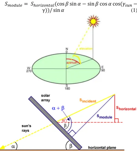
figure 1 the direct beam irradiance on an inclined surface Smodule
with module inclination (angle between surface normal and
normal through horizontal surface), orientation (angle of
horizontal offset of surface normal from south in northern hemisphere), where horizontal beam irradiance is Shorizontal, sun
elevation α (measured from horizontal surface) and sun azimuth
is sun (measured from north), is calculated by equation.
= ℎ �� � cos sin − sin cos cos −
γ / sin (1)
Figure 1: Sun’s Position and module’s orientation (Honsberg &
Bowden, 2013)
The amount of direct radiation depends on the visibility of sun at that point at any time. If the panel is visible to sun then the above mentioned equation can calculate the direct radiation for the panel if not then the panel receives only diffuse radiation. The yearly amount of direct radiation of a surface will be computed with the direct radiation taking into consideration time interval, the solar elevation and azimuth, and surface (SVF). Figure 2 shows the visibility of sky for a horizontal and a tilted module.
Figure 2: Visibility of Sky Dome (Honsberg & Bowden, 2013)
The calculation of diffuse component D is simple. From a simple model, assuming isotropic radiation from the whole sky dome, it follows that the module will receive just the proportional part of Diffuse Horizontal Irradiation (DHI) obtained by INSEL simulation engine. Equation 2 represents the diffuse radiation.
� = � ∗ �� (2)
So the total radiation Rtotal received by the module would be the summation of direct and diffuse radiation which has been represented by equation 3.
� = + � (3)
4. METHODOLOGY
Most methods calculate the direct and diffuse radiation upon a surface by measuring the tilt and orientation of the surface, solar elevation and azimuth. They do not use the effect of shadows. To calculate a realistic result including shadow, the visibility of the sun has to be measured at each point for which potential calculation has been done. This however is almost impossible. Therefore we have to select a tiny area where we think the characteristics for shadow will be same and then perform a radiation simulation. So the whole process can be spilt into two parts: 1) time independent, i.e. getting the sky visibility array for each point and 2) time dependent, i.e. simulation with the solar radiation data . The advantage of this approach is that the first part can be seen as pre-processing and can be performed only ones providing resolution of 3D models and the sky. The second part concentrates on the time resolution and allows different time intervals to be investigated.
4.1 Time independent
The time independent part defines the resolution of the sky patches and the mesh of the building geometry and computes the SVF. This is done by finding the neighborhood of buildings for shadow casting using a kd-Tree, performing ray-casting per triangle. The results stored in in binary format (true, false).
Figure 3: Processing 3D city model to make input data for Solar Potential Calculation.
Each building may have two roles. It can be: 1. A shadow caster which will block the direct radiation and/or 2. A shadow receiver which is the point we just calculated. Figure 3 illustrates the workflow of the first part. Depending on whether the building shadow caster or shadow receiver, use different
LODs. We consider that shadow casting surface doesn’t need to
have details on the facades, because a wall surface with a window and door will cast approximately the same amount of shadow if there was no door or window at all. Therefore we use LOD2 when we consider the building as shadows caster. But as for shadow receiving surface, the more detail the better. In this case the windows and the doors must be excluded from the surface since no photovoltaic cells can be placed on them. To calculate the SVF, a ray plane intersection algorithm has been used where it is possible to determine if a point is going through a triangle. And for calculating shadow receiving points, LOD3 model has been subdivided into very small triangles according to desired resolution and then the centre of the triangle has been stored.
Figure 4: Workflow for SVF calculation for each shadow receiving point.
Figure 4 shows the workflow for SVF calculation for each shadow receiving point. First step for sky model visibility is to read these sets of shadow receiving points and then to determine visibility the simple ray plane intersection algorithm is used which can check if the ray intersects a shadow casting triangle or not. This is done to find out some evenly distributed points upon the surface from where visibility is measured and the small triangle assumed to have similar visibility as the point. This calculation is done for each shadow receiving point and for each sky patch and the result is stored for each point in lookup table.
4.2 Time dependent part
In the time dependent part, the time resolution can be changed and investigated. The second time dependent part is extremely fast because uses the already computed SVF. A simulation is done for a given time stamp to get position of sun and sky patch in which sun fits in, the SVF is obtained from the lookup table.
The solar radiation will be calculated for those shadow receiving specific points distributed over the surface, which will represent the whole surface. For direct and diffuse radiation the real time sun information is used. Figure 5 illustrates the workflow of hourly solar radiation calculation for each surface for a year. More details about the methodology can be found in our previous papers (Alam, et al., 2012) (Alam, et al., 2011).
In the whole methodology, the resolution of the geometry and the time interval is of critical importance for the resulting quality and computation time. Four resolutions are considered in this paper: 1. temporal resolution, 2. object surface resolution (maximum triangle size), 3. blocking obstacle resolution (LoD1, LoD2, or LoD3), and 4. sky resolution (sky-patches used to divide the sky-dome )
Figure 5: Workflow of solar radiation calculation for each surface for a year
5. COMPARISON OF RESOLUTION
Three parameters have been compared here with different resolutions to find out the optimum with respect to result quality and computation time. Those are time interval for calculating visibility of sun, smallest size of a surface to be considered and number of the sky-patches used to divide the sky-dome.
5.1 Time interval
Usually, the solar potential needs to be computer per year. This can be done in many ways. For example monthly mean, weekly mean, daily mean hourly or even with minutely interval. But each has its own computational price. The more fine the time interval is, the more realistic is the result. But if we analyse the sun position we see that sometimes we have very similar sun position for many time instance. So if the time interval is fashioned in such a manner that there will be less repetition and more distribution then the result would be more realistic. Figure 6 shows shadow monthly variation in SVF for direct radiation and figure 7 shows hourly difference in SVF for direct radiation for one day at a part of Grünbühl City Model.
Figure 6 Differences in SVF for Direct Radiation at specific time of each month.
Figure 7 Hourly differences in Sky View Factor for Direct Radiation on a specific day
Figure 8 Comparison of distribution of sun in the Sky Patches Left: for every hour a curve is showing the sky position thought
the year (not all 24 curves visible due to night time). Right: same for every 10 minutes (again not all 24*6=144
curves visible).
This simulation has been done for hourly time interval for a whole year (24*365/2 = 4380 times, during night time computation is skipped). Figure 8 shows distribution of sun position within sky patches. In the left part of the figure is this hourly sun position during daytime for 365 days. There is a lot of sun position close to each other which means the different between their results will be very small. In the right part of the figure, time interval is 10 minutes, which is 6 times more calculation, but it is done for every 6th day so the total number of computation is almost same as before. But what we notice is the sun position distribution is much distributed than the previous option. Here are some numerical representations of the impact of time interval for 78 buildings in Finsterrot.
Figure 8 Comparison of hourly and minutely radiation calculation of the longest day of 2015 (radiation in Wm-2 on the
vertical axis)
Figure 9 Comparison of hourly and minutely radiation calculation of the shortest day of 2015 (radiation in Wm-2 on the
vertical axis)
Figure 8-9 shows a comparison between hourly and minutely radiation calculation of a part of Finsterrot model with 78 buildings with no nearby vegetation and with 600 sky patches. For longest day we see that the minutely data has more radiation than hourly data because the total amount of shadow time has been decreased because of taking small time interval. And for shortest day it has just opposite effect here so from here we can say the result is directly proportional to time interval.
5.2 Meshing resolution
Meshing is the key factor of the result. It affects the quality of result. To calculate photovoltaic potential there has to be some points for which the radiation will be calculated. This point will represent a part of surface. How big this part of surface will be is defined by a resolution. The selected options for meshing triangles are 5 sqm, 2.5 sqm, 1.25 sqm, 0.75 sqm, 0.5 sqm, 0.25 sqm, 0.1 sqm and 0.01 sqm. Figure 10 shows the result of meshing of some buildings in Grünbühl, on the left side results without showing meshing grid and on the right side with grid and at the top with 7589 triangles at very low resolution with area less than 5sqm (which means 20 points will be calculated on a 10x10 m2 surface), in the middle 28938 triangles at normal resolution with area less than 0.75 sqm (which means 12 points will be calculated on a 3x3 m2 surface) and at the bottom 3564885 triangles very high resolution with area less than 0.01 sqm (which means 100 points will be calculated on a 1x1 m2 surface). In this figure red color is shown as shadowed area and green area is where the sun is visible at a given moment in time.
Figure 10 Effect of Meshing to find shadow receiving point at different resolution (red is shadow)
Figure 11 Comparison of a meshing resolution and its effect. (radiation in Wm-2 on the vertical axis)
Figure 11 shows a comparison of meshing resolution from very low to extremely high for a part of Finsterrot model with 78 buildings with no nearby vegetation. There were significant difference between the visibility result of each time interval for each mesh but shadowed part are mostly in the morning and in the afternoon when radiation is very low so the effect dissolves a little bit here and further more when we sum up over the year the total radiation the effect dissolve even more. But still a difference is visible from the graph. And meshing resolution is also directly proportionate to the quality of result.
0
5.3 Sky patch resolution
In this research SVF play a role of pre-processor. To calculate solar radiation for a point through a whole year, an hourly estimation is necessary. But visibility calculation is a time expensive method and solar position repeats itself if an approximation is done. So for this purpose to calculate SVF the whole sky has been assumed as a dome, which is like half of a sphere. The sky dome has been divided into some almost equal area triangles. The number of triangles depends on how big the triangle has to be. It would be perfect if we could just divide it into equilateral triangles, but it is not geometrically possible. So first the dome is spit into 6 equal triangles and then the triangles are sub triangle according to need. It can be expressed by a formula mentioned in equation 4 where N is total number of triangles and n is horizontal division in the sky dome.
� = 6�2 (4)
Figure 12 Sky Dome and Sun’s position and visibility of sky patches
In the left part of figure 12 it shows only sky dome for a point on the solar panel installed on the roof of a building. Visibilities of the sky dome are saved within the point by a BitSet (Oracle, 2016), which has the size of N. The figure also shows the hourly distribution of sun onto the sky patches for the whole year. In the right part, the overlap of sun position distribution and sky patches are clearly visible. So for direct radiation only these sky patches will be checked for visibility, it also shows the visibility of sky patch through a point on the solar panel. For this point the amount of received diffuse radiation is 89% of total diffuse radiation but for direct radiation the peak sun hours are blocked when the radiation is high, so it will receive low direct radiation. Some of the well-known model uses Equal-angle Sub Division technique. But the area of the patches are different so each point the visible patches area has to be calculated and also the distribution is uneven for sun position. Because it will have more density of sun position in the morning and evening when there are more obstacles and less in the noon when sun is high and mostly visible. The influence of SVF resolution has been described in result section. Figure 13 shows hourly sun position distribution for a whole year in the left part with 24 sky patches and in the right part with 1944 sky patches. It is true that the fine the sky patch is the accurate is the sky patch selection for sun position. But it should be kept in mind that the sky patches are used to reduce calculation time and reusability. Because the use of sky patches are two fold, once for direct radiation another for diffuse radiation. If we keep making it more fine then after some time it will need more calculation time than using the actual sun position. Because for very fine sky-patches there is no reuse anymore (and computations for many patches that are never used). More/ fine sky-patches do give better estimation of SVF.
Figure 13 shows a comparison of meshing resolution from very low to extremely high for a part of Finsterrot model with 78 buildings with no nearby vegetation. And Figure 14 shows a
comparison of sky patch resolution from 150 to 600. Like the meshing resolution it is noticeable that there is a difference in result for high and low resolution of sky patch and sky patch resolution is directly proportional to the quality of result.
Figure 13 Equal-angle Sub Division of Sky Dome (ref)
Figure 14 Comparison of sky patch resolution and its effect (radiation in Wm-2 on the vertical axis)
6. SUMMARY AND FUTURE WORK
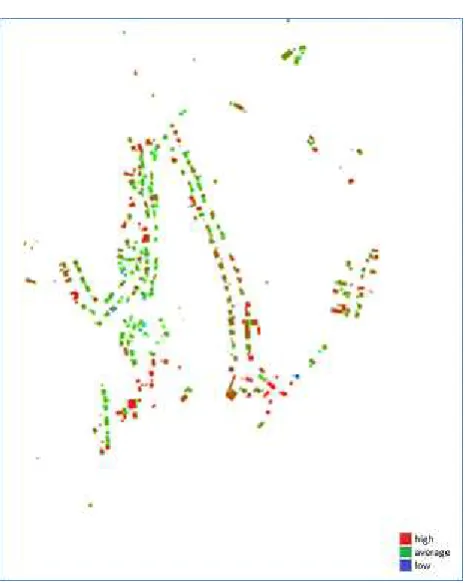
Figure 15 shows different areas in Stuttgart near Wuestenrot. Three types of result have been prepared for each part firstly radiation received by the polygons in w/m2 then after shadow by the building but without vegetation and finally with vegetation for all the models. In this paper the result from a part of Finsterrot model has been discussed. Finsterrot model has 440 buildings with 4173 polygons which include 10522 triangles.
Figure 15 Wuestenrot Map
0 5000 10000 15000 20000 25000 30000 35000
1 4 7 10 13 16 19 22 25 28 31 34 37 40 43 46 49 52 55 58 61 64 67 70 73 76
low high
Figure 16 Solar radiations on Buildings in Finsterrot
Figure 17 Finsterrot LOD 2 model with solar potential for only buildings.
Figure 16 represents a part of Finsterrot with some building with results at high resolution. Red represents most availability of sunlight, blue represents absence of sun light and green represents the average. Figure 17 represents the LOD2 model of whole Finsterrot where the buildings are marked as yellow and vegetation are green (there are more but those parts have no building, so it was ignored). Result represents the Solar Potential of only the buildings by taking vegetation also into consideration.
The methodology represents an optimum approach for calculating solar radiation distribution on roofs and wall surfaces of a 3D city model. It finds out the most suitable places to install photovoltaic modules in buildings and also helps calculating the electricity production according to the location of the photovoltaic module. Vegetation has not been taken into account and BitArray is not sufficient as crown is transparent. In our next papers we will focus on the semi-transparent vegetation object, effect of mixed LOD computation and filters to reduce computation time and also a comparison of performing calculation in CPU and GPU.
REFERENCES
Alam, N., Coors, V., Zlatanova, S. & Oosterom, P., 2011. Shadow effect on photovoltaic potentiality analysis using 3D city models, the Joint ISPRS Workshop on 3D City Modelling& Applications and the 6th 3D GeoInfo Conference, 26-28 June. Wuhan
Alam, N., Coors, V., Zlatanova, S. & Oosterom, P., 2012. Shadow effect on photovoltaic potentiality analysis using 3D city models, Int. Arch. Photogramm. Remote Sens. Spatial Inf. Sci., XXXIX-B8, 209-214. Melbourne
Catita, C., Redweik, P., Pereira, J. & Brito, M., 2014. Extending solar potential analysis in buildings to vertical facades. Computers & Geosciences, Band 66, pp. 1-12.
Freitas, S., Catita, C., Redweik, P. & Brito, M. C., 2015. Modelling solar potential in the urban environment: State-of-the-art review. Renewable and Sustainable Energy Review, Band 41, pp. 915-931.
Fu, P. & Rich, P. M., 1999. Design and Implementation of the Solar Analyst: an ArcView Extension for Modeling Solar Radiation at Landscape Scales. s.l
Gueymard, C., 1987. An anisotropic solar irradiance model for tilted surfaces and its comparison with selected engineering algorithms. Solar Energy, 38(5), pp. 367-386.
Hay, J. E., 1993. Calculating solar radiation for inclined surfaces: Practical approaches. Renewable Energy, 3(4-5), pp. 373-380.
Hofierka, J. & Kanŭk, J., β009. Assessment of photovoltaic
potential in urban areas using open-source solar radiation tools. Renewable Energy, Band 34, pp. 2206-2214.
Hofierka, J. & Suri, M., 2002. The solar radiation model for Open source GIS:implementation and applications. Trento, Italy
Honsberg, C. & Bowden, S., 2013. PVCDROM. [Online] Available at: http://pveducation.org/
[Access on 14 February 2016].
Klucher, T., 1979. Evaluation of models to predict insolation on tilted surfaces. Solar Energy, 23(2), pp. 111-114.
Moon, P. & Spencer, D., 1947. Illumination from a non-uniform sky. Trans. Illum. Eng. Soc, Volume 37, pp. 707-726.
National Ocean Service, 2015. What is LIDAR?. [Online] Available at: http://oceanservice.noaa.gov/facts/lidar.html [Access on 13 February 2016].
Nguyen, H. T. & Pearce, J. M., 2012. Incorporating shading losses in solar photovoltaic potential assessment at the municipal scale. Solar Energy, 13 Februar, pp. 1245-1260.
Oracle, kein Datum Java™ Platform. [Online]
Available at:
https://docs.oracle.com/javase/7/docs/api/java/util/BitSet.html [Access on 21 01 2016].
Perez, R. et al., 1987. A new simplified version of the perez diffuse irradiance model for tilted surfaces. Solar Energy, 39(3), pp. 221-231.
Ramírez-Faz, J., Lopez-Luque, R. & Casares,. F., 2015. Development of synthetic hemispheric projections suitable for assessing the sky view factor on vertical planes. Renewable Energy, Volume 74, pp. 279-286.
Redweik, P., Catita, C. & Brito, M., 2013. Solar energy potential on roofs and facades in an urban landscape. Solar Energy, Band 97, pp. 332-341.
Reindl, D., Beckman, W. & Duffie, J., 1990. Evaluation of hourly tilted surface radiation models. Solar Energy, 45(1), pp. 9-17.
Šúri, M. & Hofierka, J., β004. A New GIS-based Solar Radiation Model and Its Application to Photovoltaic Assessments. Transactions in GIS, 8(2), pp. 175-190.