THE ATMOSPHERIC COMPENSATION COMPONENT OF A LANDSAT LAND
SURFACE TEMPERATURE (LST) PRODUCT: ASSESSMENT OF ERRORS EXPECTED
FOR A NORTH AMERICAN TEST PRODUCT
M. J. Cook, J. R. Schott∗
Rochester Institute of Technology, Chester F Carlson Center for Imaging Science, 54 Lomb Memorial Drive, Rochester, New York 14623 - [email protected]
KEY WORDS:Landsat, Surface Temperature, Atmospheric Compensation
ABSTRACT:
The Landsat archive of thermal data (Landsats 4, 5 and 7) has gone through a rigorous calibration assessment and update. However, in order to be useful to most users the calibrated sensor reaching radiance must be corrected to surface temperatures by first compensating for atmospheric effects and then emissivity variations. The USGS is exploring the possibility of producing a LST product through a joint program with RIT (the atmospheric compensation component) and JPL (the emissivity compensation component). This paper addresses the atmospheric compensation component for an initial North American pilot study. In particular, the results of a comparison of retrieved water surface temperature (where emissivity is well known) and truth temperatures for over 800 sites are presented. The errors are broken down by cloud conditions with extremely good results for cloud-free conditions (errors less than 1K). The results of the error assessment for North America by cloud class are presented along with a discussion of potential quality data for a LST product. An initial assessment of the LST errors observed for Landsat 8 bands 10 and 11 are also presented. The next steps on this effort include testing of a global atmospheric compensation approach and full integration of the atmospheric and emissivity compensation tools into an operational LST product.
1. INTRODUCTION
Landsat is the longest set of continuously acquired, moderate res-olution satellite imagery. The fourth satellite in the family, Land-sat 4, was the first to capture single thermal band imagery begin-ning in 1982, followed by Landsat 5 and Landsat 7. Landsat 8, launched in February 2013, is the first to capture multiple thermal bands. With these four instruments, there are currently more than four million Landsat thermal images in the archive and between 990 and 1090 scenes acquired each day. The entire archive (with the exception of Landsat 8 for which work is currently ongoing) has been radiometrically calibrated and characterized so that the sensor reaching radiance values are well known. However, ra-diance values are difficult to interpret, so this large archive of thermal data is under utilized.
For most users, thermal data is more useful as a temperature value. The temperature of the land surface, the first interface be-tween the atmosphere and solid earth, is a useful metric across a large number of applications, including climatology, numeri-cal weather prediction, and agriculture. LST is difficult to mea-sure without altering the temperature of the surface and, for many investigations, these values are useful over large areas and long time scales, making LST products derived from satellite imagery an obvious answer. Most LST products are generated from mul-tiple thermal bands using a split window approach, which uti-lizes the differential absorption between adjacent thermal bands (Wan and Dozier, 1996). Conversion from thermal radiance to land surface temperature with only a single thermal band requires complete characterization of the atmosphere and known surface emissivity.
Our colleagues at the Jet Propulsion Laboratory (JPL) are work-ing to develop a high spatial resolution (100 m) surface emis-sivity product form the Advanced Spaceborne Thermal Emis-sion and Reflection (ASTER) radiometer. Currently available is
∗Corresponding author.
the North American ASTER Land Surface Emissivity Database (NAALSED), but plans are underway to extend this to include a dataset with global coverage (Hulley and Hook, 2009). Work discussed in this paper assumes the availability of an emissiv-ity product and focuses on the generation and error analysis of the atmospheric compensation component. Access to high qual-ity reanalysis data makes the atmospheric characterization for a single band product feasible.
Generating radiative transfer parameters from atmospheric com-pensation is well understood, but the methodology presented here incorporates and interpolates the reanalysis data and the auto-mates the process to generate unique values at every pixel in the scene. Previous studies indicate that the atmospheric compen-sation will be the largest source of error (i.e. larger error con-tributions than emissivity). We begin with an initial study and validation over North America, to be combined with NAALSED, and an analysis of the expected error and current suggestion for a confidence metric. This will later be extended to a global product.
2. BACKGROUND
The goal of this work is to generate, for every pixel in any Land-sat scene in the archive, the radiative transfer parameters from the atmospheric compensation and the expected uncertainty. This section aims to summarize the necessary tools and datasets used in the methodology to determine the transmission, upwelled radi-ance, and downwelled radiance for each pixel in any scene.
2.1 MODerate Resolution Atmospheric TRANsmission Ra-diative Transfer Code
MODTRAN solves the radiative transfer equation to character-ize reflections, emissions, and transmissions, among other out-puts (SSI, 2012). While the applications and uses of MODTRAN are far-reaching, for the purpose of this work, complete charac-terizations of the atmosphere (pressure, temperature, and rela-tive humidity) are input into MODTRAN, and the spectral out-puts (wavelength and radiance) are used to calculate the radiative transfer parameters.
2.2 The North American Regional Reanalysis Dataset The atmospheric profiles input into MODTRAN are subset from the North American Regional Reanalysis Dataset. Reanalysis, or retrospective-analysis, is the process of using observing sys-tems with numerical models to generate variables not easily ob-served or measured in a regular and consistent spatial and tempo-ral set (Rienecker and Gass, 2013). The National Center for Envi-ronmental Prediction (NCEP) produces the NARR dataset using radiosondes, dropsondes, pibals, aircraft and surface data, and cloud drift winds among other inputs. This work utilizes profiles provided 8 times daily at 29 specific pressure levels, with approx-imately 0.3◦(approximately 32 km at the lowest latitude) spacing covering North America in a 349 by 277 array (Shafran, 2007). The geopotential height [gpm] and specific humidity [kg/kg] pro-files are converted to geometric height [km] and relative humidity [%] and input, along with the temperature profile [K], into MOD-TRAN.
2.3 The Governing Equation
A governing equation contains all of the components that are rel-evant to the sensor reaching radiance. Equation 1 shows the gov-erning equation for a single Landsat thermal band, whereLobsλef f is the effective sensor reaching spectral radiance,LT λef fis the effective spectral radiance due to temperature, ǫis the surface emissivity of the pixel of interest,τis the transmission,Luλef fis the upwelled effective spectral radiance, andLdλef fis the down-welled effective spectral radiance.
Lobsλef f = (LT λef fǫ+ (1−ǫ)Ldλef f)τ+Luλef f (1)
The radiance due to temperature is the term that we wish to iso-late; this can be inverted to temperature through Plancks Equa-tion, as shown in Equation 2. Because this equation is not di-rectly invertible, we use a look up table. Given a radiance due to temperature, we invert to temperature with a two point linear interpolation using a look up table in 1 K increments.
LT λef f=
Therefore, we need to solve for all other components of the gov-erning equation in order to isolate and determine the radiance due to temperature. The observed radiance,Lobsλef f, is gen-erated from the digital number provided in the Landsat thermal band and the corresponding calibration coefficients in the scene metadata. For the case of this work, we assume that Landsats 4, 5, and 7 are characterized and calibrated and that this radi-ance value can be trusted without independent validation (Barsi et al., 2003) and (Padula et al., 2010). We also assume the in-corporation of the ASTER derived emissivity, which leaves only the transmission, upwelled radiance, and downwelled radiance.
These effective spectral values are those that will be generated for every pixel in the Landsat scene through the methodology de-scribed in Section 3. We also believe that this atmospheric com-pensation process contributes to the limiting factor in uncertainty in the final LST product, so the confidence metric associated with the atmospheric compensation is discussed in Section 4.
Effective spectral radiance values indicate that the spectral re-sponse function of the sensor being used, which differs slightly for each Landsat instrument, has been accounted for over the spectral range of sensitivity. This is shown in Equation 3, where Lλcould be any radiance value we consider, such as observed, upwelled, or downwelled. Effective spectral radiance values have units of Wm−2
sr−1
µm−1
. All effective spectral radiance values are considered in this process and the explicit notation will be dropped from here forward.
This methodology aims to process a single Landsat scene and generate the radiative transfer parameters, transmission, upwelled radiance, and downwelled radiance, for every pixel in the scene. This assumes the availability and incorporation of a digital ele-vation model providing the eleele-vation of each pixel in the scene. For a particular Landsat scene, the acquisition time of the scene is identified, and the appropriate NARR variables (geopotential height, specific humidity, and temperature) at the time samples before and after this acquisition time are subset to include only locations pertinent to the current scene. This generally results in between 110 and 150 points for each scene. Each variable is tem-porally interpolated to the Landsat acquisition time using a sim-ple two point linear interpolation. For examsim-ple, NARR samsim-ples from 12 Z and 15 Z would be linearly interpolated to a Landsat acquisition time of 14.3 Z.
After radiative transfer parameters have been generated such that the data cube encompasses an entire Landsat scene, operations must be performed at every pixel in the scene in order to gener-ate unique radiative transfer parameters for each pixel. For each pixel, the four most relevant NARR points (closest point in each direction) are selected and the radiative transfer parameters are piecewise linearly interpolated to the height of the current pixel at those four NARR points. This results in the radiative transfer parameters at the four closest NARR points associated with the appropriate elevation; the final step is to interpolate these values to the location of the current pixel. Shepards method was chosen as an inverse distance weighting function to interpolate the three radiative transfer parameters to the appropriate location for each pixel; for each of the four NARR points, a distance is calculated (di) based on the NARR point location (xi,yi) and the pixel loca-tion (x,y) [Equaloca-tion 6] and weighting values (wi) are calculated based on these distances [Equation 7]. These weights are used to interpolate the original values at each location (fi) to the new interpolated value at the pixel location (F) [Equation 8] (Shepard, 1968).
di= p
(x−xi)2+ (y−y
1)2 (6)
wi= d−p
i Pn
j=1d
−p j
(7)
F(x, y) =
n X
i=1
wifi (8)
This methodology results in the transmission, upwelled radiance, and downwelled radiance at every pixel in the Landsat scene.
4. RESULTS 4.1 Ground Truth Data
In order to validate our methodology, we compare the predicted temperatures from our process to ground truth water tempera-tures. We choose to validate against water temperatures because the emissivity of water is well known and because an instrument can be submerged and acclimated, so the temperature of water can be measured without the act of measuring altering the results. The measured bulk temperature still needs to be corrected to the skin or surface temperature of the water. Ground truth data for this study was provided for two sites by the Jet Propulsion Lab-oratory (Hook et al., 2007) and also derived from NOAA buoys from around the country through an accepted skin temperature correction method (Padula et al., 2010). Figure 1 shows the dis-tribution of sites used throughout the United States; sites were chosen to capture a variety of elevation, climate, and atmosphere and images were chosen to capture a variety of season and atmo-spheric condition.
4.2 Validation of Methodology
In order to validate the methodology, initially only cloud free scenes were processed. A validation dataset of 259 cloud free Landsat 5 scenes, each containing one of the validation sites shown above, were processed and the predicted temperature at the site of the validation measurement was compared to the ground truth temperature provided by JPL or determined from the NOAA buoy measurements. Error was calculated using Equation 9; note that a
Figure 1: Distribution of validation sites throughout the United States.
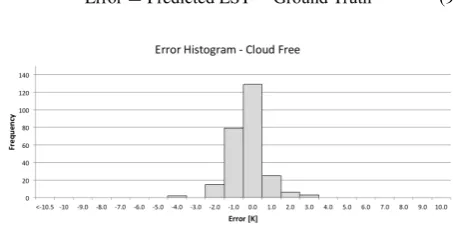
negative value indicates an underestimation by our process. Fig-ure 2 shows a histogram of error values for this cloud free Landsat 5 validation dataset.
Error=Predicted LST−Ground Truth (9)
Figure 2: Error histogram for cloud free Landsat 5 validation dataset.
Note that for the applications at which this product is aimed, 1 K to 2 K errors are generally considered acceptable. Therefore, results from this histogram are extremely encouraging. The mean error for the 259 scenes shown is -0.267 K and the standard de-viation for this dataset is 0.900 K; 90% of the dataset falls within the center three bins of the histogram with error values [-1.5 K, 1.5 K]. These results are extremely encouraging and give us con-fidence in the datasources, tools, and chosen and implemented interpolations within the process. We do acknowledge that the dataset appears to have a slight negative bias, shown both by the negative mean error and also the slight left handedness of the his-togram.
5. CONFIDENCE METRIC DEVELOPMENT
due to the inaccuracy of water vapor profiles (Cook and Schott, 2014). Because the presence of clouds is critical to understand-ing performance of the process, we turn to a more in depth cloud analysis to investigate performance of all scenes considered.
5.1 Cloud Analysis
Clouds are generally classified by height and texture. For height classifications, clouds are generally given the prefix cirro-, mean-ing high, or alto-, meanmean-ing mid. For texture classification, clouds are designated as strato-, meaning layered, uniform, widespread clouds, or cumulo-, meaning heaps of clouds or cellular, individ-ual elements. From the view of the satellite, we are currently only concerned with the texture of the clouds and therefore cre-ate two ccre-ategories: cumulus clouds, in which we group cirrocu-mulus, altocucirrocu-mulus, and other similar types, and stratus clouds, with which we group cirrostratus, altostratus, nimbostratus, and other similar types. Cirrus clouds are wispy, feathery clouds that are generally thinner but appear to exist more in layers, and are therefore included in the stratus cloud classification. For each im-age in the validation dataset, the imim-age, and more specifically the area surrounding the ground truth data point, was visually ana-lyzed and classified into one of the six categories shown in Table 1. It is important to realize that the categorization of type of cloud and in the vicinity are both subjective classifications based on the discretion of the analyst. However, all scenes in this dataset were categorized by the same analyst.
Category Description Number of Scenes
0 Cloud Free 259 [31.3%]
1 Cumulus Vicinity 98 [11.9%] 2 Stratus Vicinity 158 [19.1%] 3 Cumulus at Pixel 60 [7.3%] 4 Stratus at Pixel 202 [24.4%]
5 Cloud Covered 50 [6.0%]
Table 1: Categories used in cloud analysis and breakdown of the number of scenes in each category for the Landsat 5 validation dataset.
5.2 Cloud Analysis Results
Figure 3 is a histogram of error values for all 827 images in the validation dataset. Figure 4 shows only scenes that were cloud free at the buoy or had clouds in the vicinity of the buoy, and Figure 5 shows only scenes that were cloud free at the buoy. Note that Figure 5 is the same as Figure 2 and repeated here for ease of comparison. The numbers in the plot title indicate the cloud categorizations of the scenes included in the plot.
Figure 3: Error histogram for all images in Landsat 5 validation dataset.
Table 2 shows the mean and standard deviation of results as pixels with definite or likely cloud contamination are removed.
In Figure 3, the largest left hand bin is likely cloudy results, which we see is mostly eliminated in Figure 4. The left hand tail
per-Figure 4: Error histogram for images in cloud categories 0, 1, and 2 in the Landsat 5 validation dataset.
Figure 5: Error histogram including only scenes categorized as cloud free (0) from the Landsat 5 validation dataset.
sists in Figure 4, but note that nearly 30% of the scenes are elim-inated, and the number of scenes in the center three bins [1.5 K, 1.5 K] decreases from 395 scenes to 233 scenes, when pixels with clouds in the vicinity are removed for Figure 5. This shows that although eliminating clouds in the vicinity eliminates the left hand tail shown in the histogram, it also eliminated a large por-tion (nearly 20% of the total dataset) of good scenes. We believe that some pixels with clouds in the vicinity could still be useful to many users, with an appropriate recognition of higher potential error.
5.3 Cloud Product Incorporation
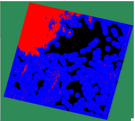
For an operational product, obviously a visual analysis of each pixel is unreasonable. Incorporation of a cloud product, and au-tomation of cloud categorization, is critical to the incorporation of the cloud analysis shown above. Landsat surface reflectance products are currently provided with a cloud mask; such a cloud mask should be provided with TM and ETM+, as well as Landsat 8 products, in the near future. Revisiting the subjective analy-sis shown above, we estimate a distance threshold of 0.5 km for cloudy pixels. That is, any ground truth site with clouds within 0.5 km (17 pixels) was classified as cloudy. Any ground truth site with clouds more than 0.5 km away but less than 5 km (167 pix-els) away was classified as having clouds in the vicinity. Finally, any ground truth site with no clouds within 5 km was classified as cloud free. One example of a cloud product is shown in Figure 6 and classification of pixels as cloudy, clouds in the vicinity, or cloud free based on the distance thresholds described above and this cloud product is shown in Figure 7.
5.4 Current Confidence Metric Suggestion
Cloud Category Mean [K] SD [K] Number of Scenes 0, 1, 2, 3, 4, 5 -8.471 19.313 826 [100%]
0, 1, 2, 3 -1.538 4.174 575 [70%]
0, 1, 2 -0.933 2.460 515 [62%]
0, 1 -0.499 2.228 357 [43%]
0 -0.267 0.900 259 [31%]
Table 2: Mean and standard deviation for groups of results as scenes with definite and then likely cloud contamination are re-moved.
Figure 6: One example of a cloud product provided with the Landsat surface reflectance product. White pixels are classified as cloudy.
Figure 7: Example of a cloud product with each pixel categorized as cloudy (red), clouds in the vicinity (blue), or cloud free (black). Note that green pixels are pixels in the surround of the image.
standard deviations would be consistent for all images based on the validation dataset, but the scene percentage is unique to this example.
Pixel Mean [K] SD [K] % of Scene
Cloud Free (Black) -0.267 0.900 13.2%
Vicinity (Blue) -1.607 3.239 65.8%
Black and Blue -0.933 2.460 86.8%
Cloudy (Red) Do Not Trust NA 21.0%
Table 3: Example of expected means and standard deviations for each category included with the additional confidence met-ric band.
6. PRODUCT EXTENSIONS
Two glaring holes in the ability of this product to be applied to ev-ery Landsat scene in the archive is the validation for other sensors as well as the extension to a global dataset. We briefly explore both in this section.
6.1 Landsat 7
A small subset of cloud free Landsat 7 scenes was processed over the same ground truth sites in order to validate the methodology for Landsat 7. The error was again calculated using Equation 9. A histogram of error values is shown in Figure 8. Only 44 cloud free Landsat 7 scenes were processed; these scenes had a mean error of -0.20 K and a standard deviation of 0.68 K. Although a larger dataset, with more variety in conditions and atmospheres, would be needed in order to more confidently validate Landsat 7, this is a good first look, and results in similar mean errors when applying the methodology to more than one sensor. This is a very encouraging initial validation.
Figure 8: Histogram of error values for small subset of cloud free Landsat 7 scenes.
6.2 Landsat 8
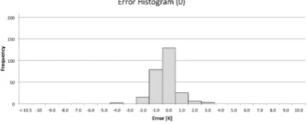
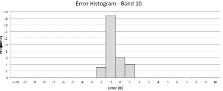
Similarly, a small cloud free dataset of Landsat 8 scenes was pro-cessed and analyzed. Although Landsat 8 has two thermal bands, and could potentially utilize a split window or other multiple ther-mal band technique, we first analyze each band separately using our single channel method. Figure 9 shows a histogram of error values for band 10 of Landsat 8 and Figure 10 shows a histogram of error values for band 11 of Landsat 8. The mean and standard deviation for each Landsat 8 band is summarized in Table 4.
Landsat 8 Mean [K] SD [K]
Band 10 -0.56 0.76
Band 11 -2.16 1.64
Table 4: Mean error and standard deviation for each band of Landsat 8.
Figure 9: Histogram of error values for small subset of cloud free Landsat 8 scenes processed using band 10.
Figure 10: Histogram of error values for small subset of cloud free Landsat 8 scenes processed using band 11.
current studies show that there are actual changes in the Landsat 8 calibration, more prevalent in band 11; it is believed that there is still currently a variable source of calibration error, correlated to scene radiance, that can be attributed to stray light from outside the detectors nominal point spread function impinging on the de-tector (Schott et al., 2014), (Montanaro et al., 2013). Therefore, these results, rather than acting as a reflection of the performance of our current methodology, will be utilized in the continuing cal-ibration work and attempts to solve the stray light problem, and a more in depth analysis of the ability to process Landsat 8 us-ing the current methodology will be revisited after there is more confidence in the calibration and characterization of the Landsat 8 thermal bands.
6.3 Global Product
As noted in Section 2.2, the current atmospheric characterization is pulled from a dataset that covers only North America. Exten-sion to a global product requires utilization of global atmospheric characterization data. The Modern-Era Retrospective Reanalysis for research and Applications (MERRA) dataset provides 1.25◦ resolution around the globe (288 by 144 array), has eight sam-ples each day, and provides variables at 42 pressure levels. The MERRA data also includes geopotential height [gpm], which we convert to geometric height [km], and temperature [K], but pro-vides the relative humidity [%], eliminating the need for conver-sion of the water vapor profile (Rienecker and Gass, 2013). These profiles are integrated into the same methodology discussed in Section 3. A small subset of the Landsat 5 validation dataset, over the same ground truth sites, was processed using the MERRA re-analysis dataset. Histograms of error values for all scenes, scenes with clouds in the vicinity or cloud free, and only cloud free scenes are shown in Figures 11, 12, and 13 respectively. The numbers in the plot title indicate the cloud categorizations in-cluded in the plot. Note that the cloud analysis of these scenes was still subjective based on analyst interpretation and not objec-tively or automatically classified as described in the cloud product incorporation.
Table 5 shows the mean and standard deviation of the subset of
Figure 11: Histogram of error values for subset of Landsat 5 val-idation dataset processed using MERRA data.
Figure 12: Histogram of error values for subset of Landsat 5 validation dataset processed using MERRA data, including only scenes with clouds in the vicinity and cloud free over the ground truth site.
Figure 13: Histogram of error values for subset of Landsat 5 validation dataset processed using MERRA data, including only scenes that are cloud free over the ground truth site.
scenes, processed using MERRA. The values shown in Table 5 are similar in magnitude to those shown in Table 2.
Therefore, these results, although an incomplete analysis, are jus-tification to move forward with a complete validation of the MERRA dataset for a global product and show very encouraging results for the ability to produce LST values for all Landsat scenes in the archive.
7. FUTURE WORK 7.1 Bias Correction
Comparison of current results for the cloud free Landsat 5 val-idation dataset shows the negative bias to be significant when compared to the Landsat 5 calibration data. Based on current calibration expectations for Landsat 5 (0.0 K±0.73 K), results
Cloud Category Mean [K] SD [K] Number of Scenes
Table 5: Categories used in cloud analysis and breakdown of the number of scenes in each category for subset of scenes processed using MERRA dataset.
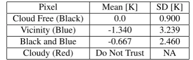
standard deviations for each category included in the confidence metric band are shown in Table 6.
Pixel Mean [K] SD [K]
Cloud Free (Black) 0.0 0.900 Vicinity (Blue) -1.340 3.239 Black and Blue -0.667 2.460 Cloudy (Red) Do Not Trust NA
Table 6: Expected means and standard deviations for each cat-egory included with the additional confidence metric band after bias correction for cloud free data.
However, analysis of our small Landsat 7 dataset shows the neg-ative bias to be insignificant. That is, based on current Landsat 7 calibration expectations (-0.05 K±0.56 K), results are not
statis-tically different at alpha level 0.05, suggesting any bias shown in these results cannot be solely attributed to our developed process. This would suggest that a bias correction to the final LST value would be inappropriate, although we recognize that this Landsat 7 dataset is also extremely small. Therefore, we intend to revisit the need for a bias correction after a more complete validation of all Landsat sensors.
7.2 Cloud Product Automation
The current confidence metric suggestion requires additional work before it can be implemented into the product. We must automate the incorporation of the cloud product and categorization of each pixel based on the distance thresholds given. With this automa-tion, we can more accurately compare our objective and subjec-tive cloud categorizations and adjust distance thresholds and ex-pected means and standard deviations accordingly. Based on a larger dataset of automated results, we can explore further im-provements. Would it be beneficial to bias pixels with clouds in the vicinity based on cloud type or distance to cloudy pixel? Is there a way to determine the type of cloud based on this cloud product and is that information useful for confidence expecta-tions? We also need to address issues with single pixels classified as clouds and how to deal with the edges of each image.
8. CONCLUSIONS
We have shown a methodology to automatically generate the ra-diative transfer parameters necessary to calculate an LST value, given the corresponding surface emissivity, for every pixel in any Landsat scene in North America. This methodology shows ex-tremely encouraging results for cloud free scenes, with a mean error when compared to ground truth data of -0.267 K, and a standard deviation of 0.900 K. With this trusted methodology, we focus on the development of a confidence metric that will prove useful to the user. Based on limitations of an initial traditional error propagation when applied to this process, and the obvious and large influence of clouds in the scene, we found that a con-fidence metric based on the proximity of cloudy pixels would be best suited for this product. We currently suggest including an ad-ditional confidence metric band, derived from the Landsat cloud
product, that categorizes each pixel as cloudy, clouds in the vicin-ity, or cloud free, with each category having some expected mean and standard deviation. Future work includes validation for all Landsat sensors and a global dataset, as well as incorporating the cloud product and improvements to the confidence metric band that could potentially provide the user with more information.
ACKNOWLEDGEMENTS
The authors would like to thank the Jet Propulsion Laboratory, NASA and USGS-EROS for their support of this work. This work is funded under NASA grant NMO710627, A Land Surface Temperature Product for Landsat.
REFERENCES
Barsi, J., Schott, J., Palluconi, F., Helder, D., Hook, S., Markham, B., Chander, G. and O’Donnell, E., 2003. Landsat tm and etm+ thermal band calibration. Can. J. Remote Sensing 29(2), pp. 141– 253.
Cook, M. J. and Schott, J. R., 2014. A novel confidence met-ric approach for a landsat land surface temperature product. In: ASPRS 2014 Annual Conference.
Hook, S. J., Vaughan, G., Tonooka, H. and Schladow, S. G., 2007. Absolute radiometric in-flight validation of mid infrared and thermal infrared data from aster and modis on the terra space-cradt using the lake tahoe, ca/nv, usa, automated validation site. IEEE Transactions on Geoscience and Remote Sensing 45(6), pp. 1798–1807.
Hulley, G. C. and Hook, S. J., 2009. The north american aster land surface emissivity database (naalsed) version 2.0. Remote Sensing of Environment 113(9), pp. 1967 – 1975.
Montanaro, M., Tesfaye, Z., Lunsford, A., Wenny, B., Reuter, D., Markham, B., Smith, R. and Thome, K., 2013. Preliminary on-orbit performance of the thermal infrared sensor (tirs) on board landsat 8. Proc. SPIE 8866, Earth Observing Systems XVIII.
Padula, F. P., Schott, J. R., Barsi, J. A., Raqueno, N. G. and Hook, S. J., 2010. Calibration of landsat 5 thermal infrared channel: updated calibration history and assesment of the errors associated with the methodology. Can. J. Remote Sensing 36(5), pp. 617– 630.
Rienecker, M. and Gass, J., 2013. Merra: Modern-era retrospective analysis for research and applications. http://gmao.gsfc.nasa.gov/research/merra/.
Schott, J. R., 2007. Remote Sensing: The Image Chain Approach. 2nd edn, Oxford Uniersity Press.
Schott, J. R., Raqueno, N., Montanaro, M., Ientilucci, E., Gerace, A. and Lunsford, A., 2014. Chasing the tirs ghosts: Calibrating the landsat 8 thermal bands. Proc. SPIE 9218, Earth Observing Systems XIX.
Shafran, P., 2007. North american regional reanalysis homepage. http://www.emc.ncep.noaa.gov/mmb/rreanl/.
Shepard, D., 1968. A two-dimensional interpolation function for irregularly-spaced data. ACM National Conference pp. 517–524.
SSI, 2012. About modtran.
http://modtran5.com/about/index.html.