Directory UMM :Data Elmu:jurnal:E:Economics Letters:Vol67.Issue1.Apr2000:

(1)

www.elsevier.com / locate / econbase

Myopia, liquidity constraints, and aggregate consumption: what

do the data say?

*

Stephen J. Perez

Economics Department, Washington State University, Pullman, WA 99164-4741, USA

Received 23 February 1999; accepted 23 September 1999

Abstract

This letter attempts to explain an apparent ‘sensitivity puzzle’ relating to US consumption data as resulting from agents who expect their income to rise over their working lives prior to retirement being liquidity constrained when young.  2000 Elsevier Science S.A. All rights reserved.

Keywords: Consumption; Liquidity constraints; Excess sensitivity

JEL classification: E21; E13; E29

1. Introduction

US consumption data appears to illustrate a ‘sensitivity puzzle.’ Predictable changes in income

affect consumption (DC /DY±_{0) violating neoclassical consumption theory. However, positive}

changes in income have a smaller effect on consumption than negative changes violating myopia and liquidity constraints. According to standard consumption theory, agents attempt to smooth consump-tion over their lifetime. Therefore, predictable changes in income should not alter consumpconsump-tion decisions. Myopia violates neoclassical consumption behavior and implies agents consume a constant proportion of their income. If an agent is unable to borrow (is liquidity constrained), he will not be able to smooth rising income but will be able to smooth falling income. Therefore, there are three

expected relationships between consumption and predictable changes in income:DC /DY50 implying

neoclassical consumption behavior, DC /DY51 implying myopia, or DC /DY50 for predictable

decreases in income and DC /DY51 for predictable increases in income.

Curiously US data show none of the above relationships. In fact, they exhibit a sort of ‘sensitivity puzzle.’ Consumption appears to respond more to predictable decreases in income than to predictable

*Tel.:11-509-335-1740; fax: 11-509-335-4362. E-mail address: sjperez@wsu.edu (S.J. Perez)

(2)

1

increases for both aggregate US data (Shea, 1995a) and for household data (Shea, 1995b). This relationship does not support neoclassical consumption, myopia, or liquidity constraints in a traditional consumption model. I propose that these results do support the existence of liquidity constraints when agents plan to retire at the end of their lifetimes.

2. How should the empirical evidence be interpreted?

In this section I describe consumption behavior that explains the sensitivity puzzle. Suppose an

agent maximizes his utility over his lifetime. Utility depends on current consumption, U(c ), with a_t

rate of time preference equal tor. The agent earns certain income, y , in each period, and can borrowt

or save at the interest rate equal to r. The consumer’s maximization problem is:

T

where A is wealth at time tt 5t. If r5r, the agent will smooth consumption over his lifetime with

ct5ct11. Expected changes in income have no effect on consumption. Suppose further that the agent

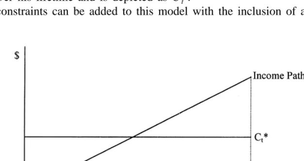
believes his income will rise, on average, over his lifetime as depicted in Fig. 1. Optimal consumption

*

is constant over his lifetime and is depicted as C .t

Liquidity constraints can be added to this model with the inclusion of another constraint

Fig. 1. Income and consumption for an unconstrained agent whose income grows over his lifetime. 1

(3)

ct#yt1At (3)

The agent would like to smooth consumption but may not be able to due to borrowing constraints. If

*

the agent is constrained, c is greater than cash on hand ( y_t _t1A ). So the agent consumes his income_t

and wealth. Once the agent’s wealth is spent he is constrained for the rest of his life until t5T. The

*

next period, c_t₁₁.c . As long as income grows over the agent’s lifetime, Fig. 1 can be used to depict_t

any period up to the point where t5T. Therefore, as Deaton (1991) showed, the consumer continues

to consume his income for the rest of his life and DC /DY51.

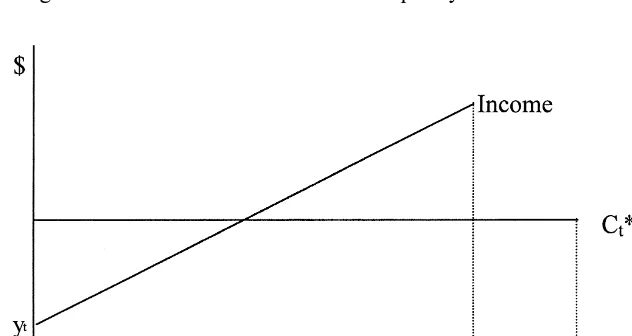
Incorporation of retirement changes this result. Suppose, each agent plans to retire at time R (see Fig. 2), changing the budget constraint:

T R

t2t t2t

O

(11r) ct5

O

(11r) yt1At (4)

t5t t5t

Under these conditions, the agent cannot continually consume his income up to time R because he will not have accumulated any assets to live off of during retirement. Eventually expected increases in income will grow higher than optimal consumption and the agent will save. Agents go through three phases of life: liquidity constrained, saving, retired.

To incorporate the possibility of business cycles, suppose the long-run path of an agent’s expected income is upward sloping as depicted in Fig. 2. However, there are expected cycles around that path as depicted in Fig. 3. Agents continue to be liquidity constrained in general when young and saving during their middle years. However, it is possible that during the liquidity constrained phase the cycles can push income in any period above optimal consumption in that period and the agent will save the

difference (DC /DY,1). Negative changes in income can never relax the liquidity constraint, but

positive changes can. Therefore, DC /DY (with DY.0),DC /DY (with DY,0).

Agents go through three phases of life: liquidity constrained, not liquidity constrained, and retired. When liquidity constrained, agents save income that relaxes the liquidity constraint. In this way, positive changes in income can relax the liquidity constraint and have a smaller effect on consumption than negative changes in income that never relax the liquidity constraint.

(4)

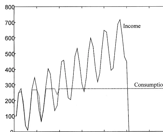
Fig. 3. Simulated income and consumption of liquidity constrained agent. Note: the figure shows income and consumption for a simulated agent who is liquidity constrained. Income follows the process: yt5yt211101150 sin(t), with y05100. Consumption is the minimum of optimal consumption and cash on hand ( yt1accumulated assets) but may not fall below zero. The agent lives for 70 years and retires after 50.

Fig. 3 shows the path of income and consumption for just such an agent. Income follows a certain

path that grows over time, but cycles around this growth path: y_t5y_t₂₁1101150 sin(t), with

y05100. Consumption is the minimum of optimal consumption (assuming r5r50) and cash on

hand ( y_t1accumulated assets) but may never fall below zero. In the simulation, the agent lives for 70

2

years, but only earns income over the first 50 years. As can be seen in the figure, the agent is liquidity constrained in the early phase of life (about the first 20 years). Eventually, the agent accumulates enough assets to smooth over both cyclical downturns and retirement. However, prior to this point, consumption tracks income very closely when income falls. Increases in income are consumed up to the point of relaxing the liquidity constraint, at which point excess income is saved.

3. Conclusion

US consumption data exhibit a ‘sensitivity puzzle:’ consumers do not consume according to neoclassical consumption behavior, myopia, or as if they are liquidity constrained. However, if the

2

(5)

standard consumption model is altered to include retirement the empirical results are not a puzzle at all. If an agent’s income rises over his working life and he plans to retire near the end of life, increases in income that relax the liquidity constraint are saved while decreases in income never relax the liquidity constraint. The response of consumption to expected reductions in current income is larger than that to expected increases in current income.

Acknowledgements

I thank Bruce Blonigen, Raymond Batina, Erick Eschker, and James Hartley for useful comments and suggestions. All errors are mine alone.

Appendix A

This is the Matlab 5.1 program used to simulated income and consumption for Fig. 3.

(6)

References

Deaton, A., 1991. Saving and liquidity constraints. Econometrica 59, 1221–1248.

Shea, J., 1995a. Myopia, liquidity constraints, and aggregate consumption: a simple test. Journal of Money, Credit, and Banking 27, 798–805.