Direction of Arrival Estimation Using the
Parameterized Spatial Correlation Matrix
Jacek Dmochowski, Jacob Benesty
, Senior Member, IEEE
, and Sofiène Affes
, Senior Member, IEEE
Abstract—The estimation of the direction-of-arrival (DOA) of one or more acoustic sources is an area that has generated much interest in recent years, with applications like automatic video camera steering and multiparty stereophonic teleconferencing entering the market. DOA estimation algorithms are hindered by the effects of background noise and reverberation. Methods based on the time-differences-of-arrival (TDOA) are commonly used to determine the azimuth angle of arrival of an acoustic source. TDOA-based methods compute each relative delay using only two microphones, even though additional microphones are usually available. This paper deals with DOA estimation based on spatial spectral estimation, and establishes the parameterized spatial cor-relation matrix as the framework for this class of DOA estimators. This matrix jointly takes into account all pairs of microphones, and is at the heart of several broadband spatial spectral estima-tors, including steered-response power (SRP) algorithms. This paper reviews and evaluates these broadband spatial spectral esti-mators, comparing their performance to TDOA-based locators. In addition, an eigenanalysis of the parameterized spatial correlation matrix is performed and reveals that such analysis allows one to estimate the channel attenuation from factors such as uncalibrated microphones. This estimate generalizes the broadband minimum variance spatial spectral estimator to more general signal models. A DOA estimator based on the multichannel cross correlation coefficient (MCCC) is also proposed. The performance of all proposed algorithms is included in the evaluation. It is shown that adding extra microphones helps combat the effects of background noise and reverberation. Furthermore, the link between accurate spatial spectral estimation and corresponding DOA estimation is investigated. The application of the minimum variance and MCCC methods to the spatial spectral estimation problem leads to better resolution than that of the commonly used fixed-weighted SRP spectrum. However, this increased spatial spectral resolution does not always translate to more accurate DOA estimation.
Index Terms—Circular arrays, delay-and-sum beamforming (DSB), direction-of-arrival (DOA) estimation, linear spatial predic-tion, microphone arrays, multichannel cross correlation coefficient (MCCC), spatial correlation matrix, time delay estimation.
I. INTRODUCTION
P
ROPAGATING signals contain much information about the sources that emit them. Indeed, the location of a signal source is of much interest in many applications, and there exists a large and increasing need to locate and track sound sources.Manuscript received September 6, 2006; revised November 8, 2006. The as-sociate editor coordinating the review of this manuscript and approving it for publication was Dr. Hiroshi Sawada.
The authors are with the Institut National de la Recherche Scientifique-Énergie, Matériaux, et Télécommunications (INRS-EMT), Université du Québec, Montréal, QC H5A 1K6, Canada (e-mail: [email protected]).
Digital Object Identifier 10.1109/TASL.2006.889795
For example, a signal-enhancing beamformer [1], [2] must con-tinuously monitor the position of the desired signal source in order to provide the desired directivity and interference sup-pression. This paper is concerned with estimating the direc-tion-of-arrival (DOA) of acoustic sources in the presence of sig-nificant levels of both noise and reverberation.
The two major classes of broadband DOA estimation techniques are those based on the time-differences-of-arrival (TDOA) and spatial spectral estimators. The latter terminology arises from the fact that spatial frequency corresponds to the wavenumber vector, whose direction is that of the propagating signal. Therefore, by looking for peaks in the spatial spectrum, one is determining the DOAs of the dominant signal sources.
The TDOA approach is based on the relationship between DOA and relative delays across the array. The problem of es-timating these relative delays is termed “time delay estimation” [3]. The generalized cross-correlation (GCC) approach of [4], [5] is the most popular time delay estimation technique. Alter-native methods of estimating the TDOA include phase regres-sion [6] and linear prediction preprocessing [7]. The resulting relative delays are then mapped to the DOA by an appropriate inverse function that takes into account array geometry.
Even though multiple-microphone arrays are commonplace in time delay estimation algorithms, there has not emerged a clearly preferred way of combining the various measurements from multiple microphones. Notice that in the TDOA approach, the time delays are estimated using onlytwomicrophones at a time, even though one usually has several more sensor outputs at one’s disposal. The averaging of measurements from indepen-dent pairs of microphones is not an optimal way of combining the measurements, as each computed time delay is derived from only two microphones, and thus often contains significant levels of corrupting noise and interference. It is thus well known that current TDOA-based DOA estimation algorithms are plagued by the effects of both noise and especially reverberation.
To that end, Griebel and Brandstein [8] map all “realizable” combinations of microphone-pair delays to the corresponding source locations, and maximize simultaneously thesum(across various microphone pairs) of cross-correlations across all pos-sible locations. This approach is notable, as it jointly maximizes the results of the cross-correlations between the various micro-phone pairs.
The spatial spectral estimation problem is well defined in the narrowband signal community. There are three major methods: the steered conventional beamformer approach (also termed the “Bartlett” estimate), the minimum variance estimator (also termed the “Capon” or maximum-likelihood estimator), and the linear spatial predictive spectral estimator. Reference [9]
provides an excellent overview of these approaches. These three approaches are unified in their use of the narrowband spatial correlation matrix, as outlined in the next section.
The situation is more scattered in the broadband signal case. Various spectral estimators have been proposed, but there does not exist any common framework for organizing these approaches. The steered conventional beamformer approach applies to broadband signals. The delay-and-sum beamformer (DSB) is steered to all possible DOAs to determine the DOA which emits the most energy. An alternative formulation of this approach is termed the “steered-response power” (SRP) method, which exploits the fact that the DSB output power may be written as a sum of cross-correlations. The computational requirements of the SRP method are a hindrance to practical implementation [8]. A detailed treatment of steered-beam-former approaches to source localization is given in [10], and the statistical optimality of the approach is shown in [11]–[13]. Krolik and Swingler develop a broadband minimum variance estimator based on the steered conventional beamformer [14], which may be viewed as an adaptive weighted SRP algorithm. There have also been approaches that generalize narrowband localization algorithms (i.e., MUSIC [15]) to broadband sig-nals through subband processing and subsequent combining (see [16], for example). A broadband linear spatial predictive approach totime delay estimationis outlined in [17] and [18]. This approach, which is limited to linear array geometries, makes use of all the channels in a joint fashion via the time delay parameterized spatial correlation matrix.
This paper attempts to unify broadband spatial spectral esti-mators into a single framework and compares their performance from a DOA estimation standpoint to TDOA-based algorithms. This unified framework is the azimuth parameterized spatial correlation matrix, which is at the heart of all broadband spa-tial spectral estimators.
In addition, several new ideas are presented. First, due to the parametrization, well-known narrowband array processing notions [19] are applied to the DOA estimation problem, gen-eralizing these ideas to the broadband case. A DOA estimator based on the eigenanalysis of the parameterized spatial corre-lation matrix ensues. More importantly, it is shown that this eigenanalysis allows one to estimate the channel attenuation from factors such as uncalibrated microphones. The existing minimum variance approach to broadband spatial spectral esti-mation is reformulated in the context of a more general signal model which accounts for such attenuation factors. Further-more, the ideas of [17] and [18] are extended to more general array geometries (i.e., circular) via the azimuth parameterized spatial correlation matrix, resulting in a minimum entropy DOA estimator.
Circular arrays (see [20]–[22], for example) offer some ad-vantages over their linear counterparts. A circular array provides spatial discrimination over the entire 360 azimuth range, which is particularly important for applications that require front-to-back signal enhancement, such as teleconferencing. Further-more, a circular array geometry allows for more compact de-signs. While the contents of this paper apply generally to planar array geometries, the circular geometry is used throughout the simulation portion.
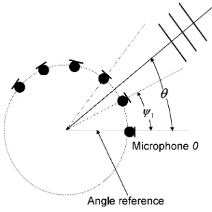
Fig. 1. Circular array geometry.
Section II presents the signal propagation model in planar (i.e., circular) arrays and serves as the foundation for the re-mainder of the paper. Section III reviews the role of the tradi-tional, nonparameterized spatial correlation matrix in narrow-band DOA estimation, and shows how the parameterized ver-sion of the spatial correlation matrix allows for generalization to broadband signals. Section IV describes the existing and pro-posed broadband spatial spectral estimators in terms of the pa-rameterized spatial correlation matrix. Section V outlines the simulation model employed throughout this paper and evaluates the performance of all spatial spectral estimators and TDOA-based methods in both reverberation- and noise-limited envi-ronments. Concluding statements are given in Section VI.
The spatial spectral estimation approach to DOA estimation has limitations in certain reverberant environments. If an inter-fering signal or reflection arrives at the array with a higher en-ergy than the direct-path signal, the DOA estimate will be false, even though the spatial spectral estimate is accurate. Such situ-ations arise when the source is oriented towards a reflective bar-rier and away from the array. This problem is beyond the scope of this paper and is not addressed herein. Rather, the focus of this paper is on the evaluation of spatial spectral estimators in noisy and reverberant environments and on their application to DOA estimation.
II. SIGNALMODEL
Assume a planar array of elements in a 2-D geom-etry, shown in Fig. 1 (i.e., circular geometry), whose outputs are denoted by , , where is the time index. Denoting the azimuth angle of arrival by , propagation of the signal from a far-field source to microphone is modeled as:
(1)
relative delay between microphones 0 and . In matrix form, the array signal model becomes:
.. .
. .. ... ..
. ... . .. ... ...
.. .
(2)
The function relates the angle of arrival to the relative delays between microphone elements 0 and , and is derived for the case of an equispaced circular array in the following manner. When operating in the far-field, the time delay between microphone and the center of the array is given by [23]
(3)
where the azimuth angle (relative to the selected angle refer-ence) of the th microphone is denoted by , , denotes the array radius, and is the speed of signal propagation. It easily follows that
(4)
It is also worth mentioning that the additive noise may be temporally correlated with the desired signal . In that case, a reverberant environment is modeled. The anechoic en-vironment is modeled by making the additive noise temporally uncorrelated with the source signal. In either case, the additive noise may be spatially correlated across the sensors.
It should also be stated that the signal model presented above makes use of the far-field assumption, in that the incoming wave is assumed to be planar, such that all sensors perceive the same DOA. An error is incurred if the signal source is actually lo-cated in the near-field; in that case, the relative delays are also a function of the range. In the most general case (i.e., a source in the near-field of a 3-D geometry), the function takes three parameters: the azimuth, range, and elevation. This paper fo-cuses on a specific subset of this general model: a source located in the far-field with only a slight elevation, such that a single parameter suffices. This is commonly the case in a teleconfer-encing environment. Nevertheless, the concepts of this paper,
although presented in far-field planar context, easily generalize to the near-field spherical case by including the range and ele-vation in the forthcoming parametrization.
III. PARAMETERIZEDSPATIALCORRELATIONMATRIX
In narrowband signal applications, a common space-time statistic is that of the spatial correlation matrix [19], which is given by
(5)
where
(6)
the superscript denotes conjugate transpose, as complex sig-nals are commonly used in narrowband applications, and de-notes the transpose of a matrix or vector. To steer these array outputs to a particular DOA, one applies a complex weight to each sensor output, whose phase performs the steering, and then sums the sensor outputs to form the output beam. Now, if the input signal is no longer narrowband, each frequency requires its own complex weight to appropriately phase-shift the signal at that frequency. In the context of broadband spatial spectral estimation, the spatial correlation matrix may be computed at each temporal frequency, and the resulting spatial spectrum is now a function of the temporal frequency. For broadband appli-cations, these narrowband estimates may be assimilated into a time-domain statistic, a procedure termed “focusing,” which is described in [24]. The resulting structure is termed a “focused covariance matrix.”
In this paper, broadband spatial spectral estimation is addressed in another manner. Instead of implementing the steering delays in the complex weighting at each sensor, the delays are actually implemented as a time-delay in the spatial correlation matrix, which is now parameterized. Thus, each microphone output is appropriately delayed before computing this parameterized spatial correlation matrix:
(7)
and real signals are assumed from this point on. The delays are a function of the assumed azimuth DOA, which becomes the parameter. The parameterized spatial correlation matrix is for-mally written as shown by (8) and (9) at the bottom of the page. The matrix is not simply the array observation matrix, as is commonly used in narrowband beamforming models. Instead, it is a parameterized correlation matrix that represents the signal
(8)
..
powers across the array emanating from azimuth . Each off-di-agonal entry in the matrix is a single cross-correlation term and a function of the azimuth angle . Notice that the various microphone pairs are combined in ajointfashion, in that altering the steering angle affects all off-diagonal entries of . This property allows for the more prudent combining of microphone measurements as compared to thead hocmethod of averaging independent pairs of cross-correlation results.
This paper relates broadband spatial spectral estimators in terms of the parameterized spatial correlation matrix
(10)
where is some estimation function, is the steered azimuth angle, and is the estimate of the broadband spatial spec-trum at azimuth angle .
The DOA estimate follows directly from the spatial spectrum, in that peaks in the spectrum correspond to assumed source locations. For the case of a single source, which is the case throughout this paper, the estimate of the source’s DOA is given by
(11)
where is the DOA estimate.
Note that this broadband extension is not without caveats: care must be taken when spacing the microphones to ensure that spatial aliasing [2] does not result.
It is also important to point out that the GCC method is quite compatible with DOA estimation based on the parameterized spatial correlation matrix—the cross-correlation estimates that comprise the matrix may be computed in the frequency-domain using a GCC variant such as the phase transform (PHAT) [4]. This paper focuses on how to extract the DOA estimate from the parameterized spatial correlation matrix; the ideas presented are general in that they do not hinge on any particular method for computing the actual cross correlations.
IV. BROADBANDSPATIALSPECTRALESTIMATORS
The following subsections detail the existing and proposed broadband spatial spectral estimation methods, relating each to the parameterized spatial correlation matrix.
A. Steered Conventional Beamforming and the SRP Algorithm
The aim of a DSB is to time-align the received signals in the array aperture, such that the desired signal is coherently summed, while signals from other directions are incoherently summed and thus attenuated. Using the model of Section II, the output of a DSB steered to an angle of arrival of is given as
(12)
The delays steer the beamformer to the desired DOA, while the beamformer weights help shape the beam accord-ingly. The weights here have been made dependent on the de-sired angle of arrival , for a reason that will become apparent in future subsections. In (12), the received signals are delayed
[or advanced, depending on the sign of ], by an amount that takes into account the array geometry, via the function .
The estimate of the spatial spectral power at azimuth angle is given by the power of the beamformer output when steered to azimuth . Therefore, to form the entire spectrum, one needs to steer the beam and compute the output power across the entire azimuth space.
The steered-beamformer spectral estimate is given by
(13)
Substitution of (12) into (13) leads to
(14)
Expression (14) may be written more neatly in matrix notation as
(15)
where
(16)
The DOA estimate is thus given by
(17)
The maximization of a steered beamformer output power is equivalent to maximizing a quadratic of the beamformer weight vector with respect to the angle of arrival. Altering the angle affects the parameter in the quadratic form, namely, the param-eterized spatial correlation matrix.
The well-known SRP algorithm [10] follows directly from a special case of (17), where for all , and is a vector
of ones:
(18)
For this special case of fixed unit weights, this means that the maximization of the power of a steered DSB is equivalent to the maximization of the sum of the entries of .
B. Minimum Variance
The minimum variance approach to spatial spectral esti-mation involves selecting weights that pass a signal [i.e., a broadband plane wave ] propagating from azimuth with unity gain, while minimizing the total output power, given by . The application of the minimum variance method to broadband spatial spectral estimation is given in [14].
The unity gain constraint proposed by [14] is
(19)
and the vector follows from the fact that the signal is already time-aligned across the array before minimum variance pro-cessing. It is as if the signal is coming from the broadside of a linear array.
Using the method of Lagrange multipliers in conjunction with the cost function , the minimum variance weights become
(20)
The resulting minimum variance spatial spectral estimate is found by substituting the weights of (20) into the cost function:
(21)
The broadband minimum variance DOA estimator is thus given by
(22)
The next section presents a new idea: the eigenanalysis of the parameterized spatial correlation matrix.
C. Eigenanalysis of the Parameterized Spatial Correlation Matrix
Using the signal model of Section II, notice that when the steered azimuth matches the actual azimuth , the parameter-ized spatial correlation matrix may be decomposed into signal and noise components in the following manner:
(23)
where is the signal power
(24)
and
(25)
Note that it has been implicitly assumed that the desired signal is wide-sense stationary, zero-mean, and temporally uncorrelated with the additive noise. Consider only the signal component of . It may be easily shown that this matrix has one nonzero eigenvector, that eigenvector being , with the corresponding eigenvalue being . The vector of attenuation constants is generally unknown; however, from the above discussion, it
is apparent that the vector may be estimated from the eigenanal-ysis of .
To that end, consider another adaptive weight selection method, which follows from the ideas of narrowband beam-forming [19]. This weight selection attempts to nontrivially maximize the output energy of the steered-beamformer for a given azimuth
(26)
subject to
(27)
It is well known that the solution to the above constrained opti-mization is the vector that maximizes the Rayleigh quotient [2] , which is in turn given by the eigenvector corresponding to the maximum eigenvalue of . The resulting spatial spectral estimate is given by
(28)
where is the maximum eigenvalue of , and is the corresponding eigenvector. The DOA estimation involves searching for the angle that produces the largest maximum eigenvalue of :
(29)
In addition to producing another spatial spectrum estimate, the above eigenanalysis allows one to estimate:
(30)
Now that an estimate of the attenuation vector is available, the minimum variance method of [14] may be improved to re-flect the presence of channel attenuation factors, which were omitted in the developments of Section IV-B.
D. Improved Minimum Variance
The broadband minimum variance spatial spectral estimation proposed by [14] assumes that the attenuation vector is equal to , or a scaled version of . In practice, it is not uncommon for this assumption to be violated by factors such as uncalibrated microphones, for example. To that end, the unity gain constraint proposed by [14] is modified to reflect the more general signal model of Section II.
Taking into account the channel attenuation vector , the pro-posed unity gain constraint is
(31)
which may be simplified and written in vector notation as
(32)
Therefore, the optimal minimum variance weights become
The resulting proposed minimum variance spatial spectral esti-mate is found by substituting the weights of (33) into the cost function
(34)
The proposed broadband minimum variance DOA estimator is thus given by
(35)
E. Linear Spatial Prediction and the Multichannel Cross-Correlation Coefficient
Spatial spectral estimation using linear prediction is well de-fined for the case of narrowband signals, as the narrowband as-sumption allows one to write one of the microphone outputs as a complex-weighted linear combination of the other microphone outputs [2]. To extend this idea to the broadband case, the same method as that of the previous sections is used, in that the time delay is applied prior to computing the predictive coefficients.
This concept was first presented in [17] and [18] in the con-text of time delay estimation; the approach was limited to linear array geometries, and yielded only a single relative delay. This section generalizes the idea to planar array geometries, trans-forming the problem from time delay estimation to DOA esti-mation.
The idea is to predict, using real predictive coefficients, the output of using a linear combination of , . Using a spatial autoregressive (AR) model, the linear predictive framework is given by
(36)
where may be interpreted as either the spatially white noise that drives the AR model, or the prediction error. For each in the azimuth space, one finds the weight vector
(37)
which minimizes the criterion
(38)
subject to the constraint
(39)
where
(40)
Using the method of Lagrange multipliers, the optimal predic-tive weights are given by
(41)
and the resulting minimum mean-squared error (mmse) is
(42)
Note that both the optimal predictive coefficients and the mmse are a function of the steered angle .
The classical approach to spectral estimation using linear pre-diction is to map the optimal predictive coefficients to an AR transfer function. However, it is well known that this method is very sensitive to the presence of additive noise in the obser-vations [2]. This is because the AR model breaks down when additive noise is present. To that end, a more robust implemen-tation of linear spatial prediction is proposed in [17] and [18]. The idea is to not estimate an AR spectrum, but rather to find the parameter (i.e., the angle ) that minimizes the prediction error. In [17] and [18], the idea of linear spatial prediction was used to derive the (time delay parameterized) multichannel cross cor-relation coefficient (MCCC) in the context of linear array time delay estimation. These ideas are now extended to planar array geometries, and the azimuth angle-parameterized MCCC is pre-sented as another broadband spatial spectral estimator.
The matrix may be factorized as [17], [18]:
(43)
where
..
. . .. . .. ...
(44) is a diagonal matrix
..
. . .. . .. ... (45)
is a symmetric matrix, and
(46) is the cross-correlation coefficient between and
.
The azimuth-angle dependent mmse may be written using (43) as
where is the submatrix formed by removing the first row and column from , and stands for “determinant.” It is shown in [17] and [18] that
(48)
and thus the following relationship is established:
(49)
From this relationship, it is easily observed that minimizing the spatial prediction error corresponds to minimizing the quan-tity . Notice that when every entry of
is equal to unity (i.e., perfectly correlated microphone sig-nals). Conversely, in the case of mutually uncorrelated micro-phone outputs, . Putting all of this together, the azimuth angle parameterized MCCC is defined as
(50)
The MCCC broadband spatial spectral estimate is given by
(51)
from which the DOA estimation easily follows as
(52)
It is interesting to note that even though the linear spatial pre-dictive approach is used here to arrive at the azimuth parame-terized MCCC estimator, maximizing the MCCC actually cor-responds more closely to the minimization of the joint entropy of the received signals [28], assuming that the signals are jointly Gaussian distributed. This follows from the fact that for jointly Gaussian distributed , the joint entropy of is directly proportional to [28].
V. SIMULATIONEVALUATION
A. Simulation Environment
The various broadband spatial spectral estimators are eval-uated in a computer simulation. An equispaced circular array of three to ten omnidirectional microphones is employed as the spatial aperture. The radius of the array is chosen as the distance that fulfills the spatial aliasing equality for circular arrays. In other words, the array radius is made as large as possible without suffering from spatial aliasing [23]
(53)
where denotes the highest frequency of interest, and is chosen to be 4 kHz in the simulations. For a ten-element cir-cular array, the array radius becomes 6.9 cm. The signal sources are omnidirectional point sources. This means that the
direct-path component is stronger than any individual reflected com-ponent—as mentioned in the Introduction, it is beyond the scope of this paper to handle cases where due to source directivity and orientation, a reflected component contains more energy than the direct-path component.
A reverberant acoustic environment is simulated using the image model method [29]. The simulated room is rectangular with plane reflective boundaries (walls, ceiling, and floor). Each boundary is characterized by a frequency-independent uniform reflection coefficient which does not vary with the angle of in-cidence of the source signal.
The room dimensions in centimeters are (304.8, 457.2, 381). The circular array is located in the center of the room: the center of the array sits at (152.4, 228.6, 101.6). Two distinct scenarios are simulated, as described below.
The speaker is immobile and situated at (254, 406.4, 101.6) and (254, 406.4, 152.4) in the first and second simulation scenarios, respectively. The immobility of the source means that the evaluation does not consider frames during which the source exhibits movement. The correct azimuth angle of arrival is 60 . The distance from the center of the array to the source is 204.7 cm.
The SNR at the microphone elements is 0 dB. Here, SNR refers to spatially white sensor noise in the first scenario and spherically isotropic (diffuse) noise in the second scenario. The generation of spherically isotropic noise is performed by trans-forming a vector of uncorrelated Gaussian random variables into a vector of correlated (i.e., according to a given covariance ma-trix) Gaussian random variables by premultiplying the original (uncorrelated) vector with the Cholesky factorization [30] of the covariance matrix of a diffuse noise field [2]. The covari-ance matrix of the diffuse noise field is computed by averaging over the entire frequency range (300–4000 Hz). For the compu-tation of the SNR, the signal component includes reverberation. In terms of reverberation, three levels are simulated for each sce-nario: anechoic, moderately reverberant, and highly reverberant. The reverberation times are measured using the reverse-time in-tegrated impulse response method of [31]. The frequency-inde-pendent reflection coefficients of the walls and ceiling are ad-justed to achieve the desired level of reverberation: a 60-dB re-verberation decay time of 300 ms for the moderately reverberant case, and 600 ms for the highly reverberant case.
In the first simulation scenario, the microphones are all per-fectly calibrated with unity gains. In the second simulation sce-nario, the presence of uncalibrated microphones is simulated, by setting , to a uniformly distributed random number over the range (0.2, 1).
The source signal is convolved with the synthetic impulse re-sponses. Appropriately scaled temporally white Gaussian noise is then added at the microphones to achieve the required SNR. The microphone outputs are filtered to the 300–4000-Hz range prior to processing.
Throughout the simulations, the parameterized spatial corre-lation matrix is estimated once per frame by time-averaging
(54)
where is the time-averaged estimate of the correlation ma-trix . For all algorithms, the spatial spectrum is estimated every degree over the range (0, 359) degrees.
The planar signal model assumed in Section II results in ele-vation ambiguity in a three-dimensional environment. The sim-ulations do not take elevation into account, even though the height of the source (i.e., 1.52 m) does not equal the height of the planar array (i.e., 1.02 m) in the second simulation scenario. Notice that in a teleconferencing environment, the sources are commonly only slightly elevated compared to the array.
B. Performance Criteria
The estimated spatial spectra are plotted to observe mainlobe width and background values. These spectra are averaged over the frames and normalized such that the peak of the averaged spectrum is 0 dB.
For each simulation, the algorithms are also evaluated from a DOA estimation standpoint using the percentage of anoma-lies (estimates that differ from the actual angle of arrival by more than 5 ), and root-mean-square (rms) error measure for the nonanomalous estimates
(55)
where is the set of all nonanomalous estimates, is the number of elements in , and the prime operator is included to take into account the cyclicity of the angular space
if
if
(56)
C. TDOA Comparison Algorithm
The DOA estimation performance of the broadband spatial spectral estimators is compared to that of a standard two-step TDOA algorithm which consists of computing unweighted cross correlations in the first-step, and least-squares DOA estimation (translation of relative delays to DOA) in the second step. Formally, the algorithm computes the time delay between microphone 0 and microphone for as
(57)
and then translates these relative delays to the azimuth angle of arrival using the least-squares criterion [32], [33]
(58)
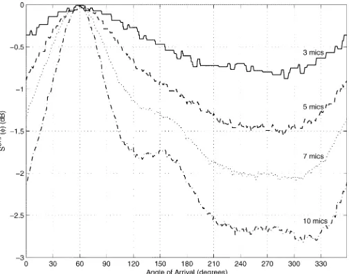
Fig. 2. SRP spatial spectral estimates for simulation scenario 1, with speech signal and moderate reverberation.
The computational requirements of TDOA-based algorithms are lower than that of the methods presented in this paper. Note that both approaches (TDOA-based and spectral estimation-based) use the cross-correlation measurements for each micro-phone pair and these cross correlations are computed over the range of physically realizable relative delays. The difference between the approaches lies in the manner in which these measurements are utilized. TDOA-based approaches simply compute the lag which produces the peak in cross correla-tion for each microphone pairing and use these optimal lags to arrive at an estimate of the DOA via an intersection or least-squares procedure. On the other hand, spatial spectral estimaton-based methods use all cross-correlation measure-ments (i.e., not just the peak values and their lag argumeasure-ments) to form the parameterized spatial correlation matrix at each DOA, followed by a search procedure over the DOA space that identifies the peak in the spectrum. The computational re-quirements of this search process are a disadvantage of spatial spectral-based methods.
D. Discussion
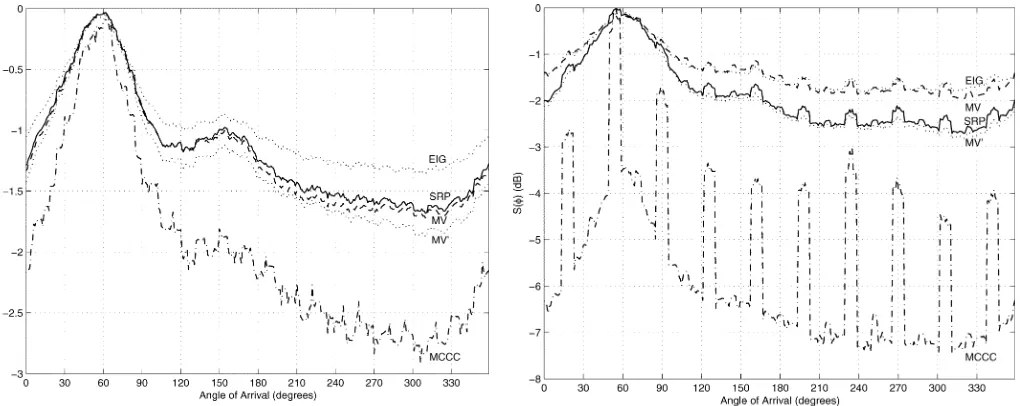
Consider first Figs. 2–5. From these figures, it is evident that adding extra microphones improves the resolution of all broadband spatial spectra. The main lobe is narrowed, and the background level, which corresponds to the power of the re-verberant field, is lowered. Thus, it is inferred that the addition of microphones combats the effects of reverberation as well as noise. A lower reverberant field level decreases the probability of anomalies.
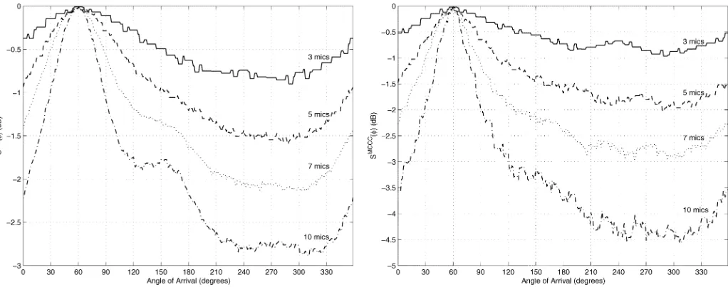
Fig. 3. Minimum variance (MV) spatial spectral estimates for simulation sce-nario 1, with speech signal and moderate reverberation.
Fig. 4. Eigenvalue spatial spectral estimates for simulation scenario 1, with speech signal and moderate reverberation.
variance weights of (20) and (33) are simply uniform (as in the SRP spectrum). Notice also that for a spatially white noise field, parametrization of the matrix does not alter the noise statistics: the time-shifting alters the off-diagonal elements only, which are all equal to zero with or without time-aligning. The eigenvalue spectrum offers the poorest resolution; however, the main idea behind the eigenanalysis of is to provide an estimate of , not to act as a spatial spectral estimator. Nevertheless, the eigenvalue spectrum may be thought of as an “intermediate” spectrum.
Consider now the spatial spectral estimates from the second simulation scenario, shown in Figs. 9–11. First of all, it is ev-ident that Krolik’s minimum variance method [14] fails in the presence of uncalibrated microphones—in fact, the “minimum variance” spectrum actually shows a higher background level than the SRP spectrum. The mismatch in the steering vector
Fig. 5. MCCC spatial spectral estimates for simulation scenario 1, with speech signal and moderate reverberation.
Fig. 6. Spatial spectral estimates for simulation scenario 1, with speech signal and no reverberation.
Fig. 7. Spatial spectral estimates for simulation scenario 1, with speech signal and moderate reverberation.
Fig. 8. Spatial spectral estimates for simulation scenario 1, with speech signal and heavy reverberation.
diffuse noise is temporally white (which is often the case with diffuse noise):
(59)
where is the noise variance, and is the identity matrix. The equation above holds strictly for circular arrays, but not linear arrays. When steering to the broadside of a linear array, there is no time-alignment necessary, and thus the spatial correlation of the diffuse noise remains. Due to the spatial decorrelation created by the parametrization, the weights of (33) are approxi-mately equal to
(60)
The minimum variance coefficients vary only to the extent of the nonuniformity of the attenuation factors, and thus the MV’
Fig. 9. Spatial spectral estimates for simulation scenario 2, with speech signal and no reverberation.
Fig. 10. Spatial spectral estimates for simulation scenario 2, with speech signal and moderate reverberation.
spectrum offers only a small benefit over the SRP spectrum. Moreover
(61)
and thus the eigenvalue spectrum closely resembles the MV’ spectrum at angles near the actual azimuth angle of arrival. Lastly, it is apparent that the MCCC spectrum is somewhat sen-sitive (i.e., the presence of deep ridges in spectrum) to factors such as variable microphone gains and source elevation.
It is important to analyze the relationship between spatial spectral estimation and DOA estimation—for example, it is interesting to investigate if the spatial spectral estimators that show a greater resolution (i.e., minimum variance, MCCC) lead to greater DOA estimation accuracy.
Fig. 11. Spatial spectral estimates for simulation scenario 2, with speech signal and heavy reverberation.
TABLE I
PERCENTAGE OFANOMALIES FORSIMULATIONSCENARIO1: SPATIALLY
WHITENOISE, NOSOURCEELEVATION, UNIFORMMICROPHONE
GAINS, TENMICROPHONES
TABLE II
RMS ERRORVALUES FORSIMULATIONSCENARIO1: SPATIALLYWHITENOISE, NOSOURCEELEVATION, UNIFORMMICROPHONEGAINS, TENMICROPHONES
spectral estimation methods in the first simulation scenario. It is obvious from the tables that the TDOA-based method provides very poor performance in reverberant conditions, as the class of spatial spectral estimators greatly outperforms the TDOA-based approach in all but the anechoic white signal case. This lends credence to the notion that jointly utilizing multiple microphone pairs combats reverberation, not just background noise. In the TDOA two-step method, a “hard-decision” is made in the com-putation of each , and thus if this decision is incorrect, the error is propagated to the least-squares stage. On the other hand, spatial spectral estimators do not make such hard decisions. In-stead, the decision is deferred until after the contribution of all microphone pairs. As expected, the SRP, MV, and MV’ methods
TABLE III
PERCENTAGE OFANOMALIES FORSIMULATIONSCENARIO2: SPHERICALLY
ISOTROPICNOISE, SOURCEELEVATED, VARIABLEMICROPHONE
GAINS, TENMICROPHONES
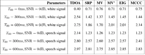
TABLE IV
RMS ERRORVALUES FORSIMULATIONSCENARIO2: SPHERICALLY
ISOTROPICNOISE, SOURCEELEVATED, VARIABLEMICROPHONE
GAINS, TENMICROPHONES.
show virtually identical performance. The slight advantage of the SRP algorithm in the heavily reverberant speech case fol-lows from the fact that the SRP algorithm does not suffer from the desired signal cancelation phenomenon. Furthermore, it is evident that the increased spatial resolution of the MCCC esti-mate does not translate to a greater DOA estimation accuracy. In fact, the MCCC spectrum exhibits anomalies in conditions where the SRP and minimum variance algorithms do not. The sensitivity of the MCCC spectrum to speech occurs due to the fact that speech is not well modeled by a Gaussian distribution, and thus, the determinant of the parameterized spatial correla-tion matrix no longer equals the joint entropy of the observa-tions. This is well explained in [28].
from (61), the DOA estimation performance of the two methods is identical (from Tables I–IV).
Recently, experiments employing real data obtained from the IDIAP Smart Meeting Room database have been performed. In these experiments, the MCCC method was shown to yield the lowest anomaly rate among the various DOA estimators.
VI. CONCLUSION
The parametrization of the spatial correlation matrix gener-alizes narrowband spatial spectral estimation methods to the broadband environment. The parametrization spatially decor-relates noise fields, and if the noise is temporally white, the noise component of the parameterized spatial correlation ma-trix is simply the identity mama-trix. As a result, the application of minimum variance spectral estimation to the broadband spatial spectral estimation problem yields only marginal gains. On the other hand, the MCCC spatial spectrum produces a significantly higher resolution than SRP and minimum variance methods.
The addition of extra microphones increases the resolution of all spatial spectral estimation methods. The eigenanalysis of the parameterized spatial correlation matrix allows one to estimate the channel attenuation vector, and is useful for determining the microphone gains.
DOA estimation methods based on spatial spectral estima-tion provide a superior performance over TDOA-based methods due to the nature of the combining of the various microphone pairs. The application of higher resolution spatial spectral esti-mation such as the minimum variance and MCCC methods to the DOA estimation problem generally yields equivalent per-formance compared to the fixed-weighted SRP method in ane-choic and moderately reverberant environments, and worse per-formance in heavily reverberant environments. In the case of the minimum variance method, the latter degradation stems from the desired signal cancellation that occurs due to reverberation; for the MCCC method, the performance degradation follows from the sensitivity of the MCCC to practical factors such as the non-Gaussian nature of speech.
ACKNOWLEDGMENT
The authors would like to thank J. Chen and Y. Huang for providing helpful suggestions and feedback regarding the sim-ulation portion of this paper. They would also like to thank the anonymous reviewers for improving the clarity and quality of the manuscript.
REFERENCES
[1] B. D. Van Veen and K. M. Buckley, “Beamforming: A versatile approach to spatial filtering,”IEEE Acoust., Speech, Signal Process. Mag., vol. 5, no. 2, pp. 4–24, Apr. 1988.
[2] D. E. Dudgeon and D. H. Johnson, Array Signal Processing. Engle-wood Cliffs, NJ: Prentice-Hall, 1993.
[3] J. Chen, J. Benesty, and Y. Huang, “Time delay estimation in room acoustic environments: An overview,” EURASIP J. Appl. Signal Process., vol. 2006, p. 19, 2006.
[4] C. H. Knapp and G. C. Carter, “The generalized correlation method for estimation of time delay,”IEEE Trans. Acoust., Speech, Signal Process., vol. ASSP-24, no. 4, pp. 320–327, Aug. 1976.
[5] M. Omologo and P. Svaizer, “Use of the crosspower-spectrum phase in acoustic event location,”IEEE Trans. Speech Audio Process., vol. 5, no. 3, pp. 288–292, May 1997.
[6] M. S. Brandstein and H. F. Silverman, “A robust method for speech signal time-delay estimation in reverberant rooms,” inProc. IEEE Int. Conf. Acoust. Speech, Signal Process., 1997, pp. 375–378.
[7] J. P. Ianiello, “High-resolution multipath time delay estimation for broad-band random signals,” IEEE Trans. Acoust., Speech, Signal Process., vol. 36, no. 2, pp. 320–327, Mar. 1988.
[8] S. M. Griebel and M. S. Brandstein, “Microphone array source local-ization using realizable delay vectors,” inProc. IEEE Workshop Ap-plicat. Signal Process. Audio Acoust., 2001, pp. 71–74.
[9] D. H. Johnson, “The application of spectral estimation methods to bearing estimation problems,” Proc. IEEE, vol. 70, no. 9, pp. 1018–1028, Sep. 1982.
[10] J. Dibiase, H. F. Silverman, and M. S. Brandstein, “Robust localization in reverberant rooms,” inMicrophone Arrays: Signal Processing Tech-niques and Applications, M. S. Brstein and D. B. Ward, Eds. Berlin, Germany: Springer-Verlag, 2001, pp. 157–180.
[11] W. Bangs and P. Schultheis, “Space-time processing for optimal pa-rameter estimation,” inSignal Processing, J. Griffiths, P. Stocklin, and C. V. Schooneveld, Eds. New York: Academic, 1973, pp. 577–590. [12] G. Carter, “Variance bounds for passively locating an acoustic source
with a symmetric line array,”J. Acoust. Soc. Amer., vol. 62, pp. 922–926, Oct. 1977.
[13] W. Hahn and S. Tretter, “Optimum processing for delay-vector estima-tion in passive signal arrays,”IEEE Trans. Inf. Theory, vol. IT-19, no. 5, pp. 608–614, Sep. 1973.
[14] J. Krolik and D. Swingler, “Multiple broad-band source location using steered covariance matrices,”IEEE Trans. Acoust., Speech, Signal Process., vol. 37, no. 10, pp. 1481–1494, Oct. 1989.
[15] R. O. Schmidt, “Multiple emitter location and signal parameter estima-tion,”IEEE Trans. Antennas Propag., vol. AP-34, no. 3, pp. 276–280, Mar. 1986.
[16] F. Asanoet al., “Real-time sound source localization and and sepa-ration system and its application to automatic speech recognition,” in
EUROSPEECH, 2001, pp. 1013–1016.
[17] J. Chen, J. Benesty, and Y. Huang, “Robust time delay estimation exploiting redundancy among multiple microphones,”IEEE Trans. Speech Audio Process., vol. 11, no. 6, pp. 549–557, Nov. 2003. [18] J. Benesty, J. Chen, and Y. Huang, “Time-delay estimation via
linear interpolation and cross-correlation,”IEEE Trans. Speech Audio Process., vol. 12, no. 5, pp. 509–519, Sep. 2004.
[19] H. Krim and M. Viberg, “Two decades of array signal processing re-search: The parametric approach,”IEEE Signal Process. Mag., vol. 13, no. 4, pp. 67–94, Jul. 1996.
[20] H. Teutsch and W. Kellermann, “EB-ESPRIT: 2D localization of mul-tiple wideband acoustic sources using eigen-beams,” inProc. IEEE Int. Conf. Acoust. Speech, Signal Process., 2005, vol. 3, pp. 89–92. [21] I. Tashev and H. S. Malvar, “A new beamformer design for microphone
arrays,” inProc. IEEE Instrum. Meas. Technol. Conf., 2005, vol. 3, pp. 18–23.
[22] A. M. McKee and R. A. Goubran, “Sound localization in the human thorax,” inProc. IEEE Int. Conf. Acoust. Speech, Signal Process., 2005, vol. 1, pp. 16–19.
[23] R. A. Monzingo and T. W. Miller, Introduction to Adaptive Arrays. Raleigh, NC: SciTech, 2004.
[24] H. Wang and M. Kaveh, “Coherent signal-subspace processing for the detection and estimation of angles of arrival of multiple wideband sources,”IEEE Trans. Acoust., Speech, Signal Process., vol. ASSP-33, no. 8, pp. 823–831, Aug. 1985.
[25] D. N. Zotkin and R. Duraiswami, “Accelerated speech source localiza-tion via a hierarchical search of steered response power,”IEEE Trans. Speech Audio Process., vol. 12, no. 5, pp. 499–508, Sep. 2004. [26] A. Johansson and S. Nordholm, “Robust acoustic direction of arrival
estimation using Root-SRP-PHAT, A realtime implementation,” in
Proc. IEEE Int. Conf. Acoust. Speech, Signal Process., 2005, vol. 4, pp. 933–936.
[27] B. Mungamuru and P. Aarabi, “Enhanced sound localization,”IEEE Trans. Syst., Man, Cybern. B: Cybern., vol. 34, no. 3, pp. 1526–1540, Jun. 2004.
[28] J. Benesty, Y. Huang, and J. Chen, “Time delay estimation via min-imum entropy,”IEEE Signal Process. Lett., vol. 14, pp. 157–160, Mar. 2007.
[29] J. B. Allen and D. A. Berkley, “Image method for efficiently simulating small-room acoustics,”J. Acoust. Soc. Amer., vol. 65, pp. 943–950, Apr. 1979.
[30] J. E. Gentle, “Cholesky factorization,” inNumerical Linear Algebra for Applications in Statistics. Berlin, Germany: Springer-Verlag, 1998, pp. 93–95.
[31] M. R. Schroeder, “New method for measuring reverberation time,”J. Acoust. Soc. Amer., vol. 37, pp. 409–412, 1965.
[32] Y. Huang, J. Benesty, and J. Chen, Acoustic MIMO Signal Pro-cessing. Berlin, Germany: Springer-Verlag, 2006.
Jacek Dmochowskiwas born in Gdansk, Poland, in December 1979. He received the B.Eng. degree (with high distinction) in communications engineering and the M.A.Sc. degree in electrical engineering from Carleton University, Ottawa, ON, Canada, in 2003 and 2005, respectively. He is currently pursuing the Ph.D. degree at the Institut National de la Recherche Scientifique-Énergie, Matériaux, et Télécommunications (INRS-EMT), Université du Québec, Montréal, QC, Canada.
His research interests are in the area of multi-channel digital signal processing, and include microphone array beamforming and source localization.
Mr. Dmochowski is the recipient of the Ontario Graduate Scholarship (2004–2005), and the National Science and Engineering Research Council Post Graduate Scholarship at the Doctoral Level (2005–2008).
Jacob Benesty(M’92–SM’04) was born in 1963. He received the M.S. degree in microwaves from Pierre and Marie Curie University, Paris, France, in 1987, and the Ph.D. degree in control and signal processing from Orsay University, Orsay, France, in 1991.
During his Ph.D. program (from November 1989 to April 1991), he worked on adaptive filters and fast algorithms at the Centre National d’Etudes des Telecommunications (CNET), Paris. From January 1994 to July 1995, he worked at Telecom Paris Uni-versity on multichannel adaptive filters and acoustic echo cancellation. From October 1995 to May 2003, he was first a Consultant and then a Member of the Technical Staff at Bell Laboratories, Murray Hill, NJ. In May 2003, he joined the Institut National de la Recherche Scien-tifique-Énergie, Matériaux, et Télécommunications (INRS-EMT), Université du Québec, Montréal, QC, Canada, as an Associate Professor. His research interests are in signal processing, acoustic signal processing, and multimedia communications. He coauthored the booksAcoustic MIMO Signal Processing
(Springer-Verlag, 2006) and Advances in Network and Acoustic Echo Can-cellation(Springer-Verlag, 2001). He is also a coeditor/coauthor of the books
Speech Enhancement(Spinger-Verlag, 2005),Audio Signal Processing for Next Generation Multimedia Communications System (Kluwer, 2004), Adaptive Signal Processing: Applications to Real-World Problems (Springer-Verlag, 2003), andAcoustic Signal Processing for Telecommunications(Kluwer, 2000). Dr. Benesty received the 2001 Best Paper Award from the IEEE Signal Processing Society. He was a member of the editorial board of the EURASIP Journal on Applied Signal Processing and was the Co-Chair of the 1999 International Workshop on Acoustic Echo and Noise Control.
Sofiène Affes(M’94–SM’04) received the Diplôme d’Ingénieur in electrical engineering and the Ph.D. degree (with honors) in signal processing from the École Nationale Supérieure des Télécommunica-tions (ENST), Paris, France, in 1992 and 1995, respectively.
He has been with Institut National de la Recherche Scientifique-Énergie, Matériaux, et Télécommunica-tions (INRS-EMT), Université du Québec, Montréal, QC, Canada, as a Research Associate from 1995 until 1997, then as an Assistant Professor until 2000. Cur-rently, he is an Associate Professor in the Personal Communications Group. His research interests are in wireless communications, statistical signal and array processing, adaptive space-time processing, and MIMO. From 1998 to 2002, he has been leading the radio design and signal processing activities of the Bell/Nortel/NSERC Industrial Research Chair in Personal Communications at INRS-ÉMT. Currently, he is actively involved in a major project in wireless of PROMPT-Québec (Partnerships for Research on Microelectronics, Photonics and Telecommunications).