O R I G I N A L P A P E R
The Ore Grade and Depth Influence on Copper Energy Inputs
R. H. E. M. Koppelaar1,2 •H. Koppelaar3
Received: 15 March 2016 / Accepted: 12 November 2016
The Author(s) 2016. This article is published with open access at Springerlink.com
Abstract The study evaluated implications of different ore grades and mine-depth on the energy inputs to extract and process copper. Based on a 191 value dataset from 28 copper mining operations, seven model equations explaining operational energy costs were statistically evaluated. Energy costs for copper mines with leaching operations were not found to be significantly affected by ore grades nor mine-depth as all tested equations were rejected in the analysis. In case of mines with milling/ flotation operations, a significant relation was established (p\0.000,R2=0.63 for surface mines andR2=0.84 for underground mines) which was found to be: energy cost is log-linearly dependent on depth plus the reciprocal of ore grade. On the basis of the equation, an ore grade of 0.5, 0.4 and 0.3% at 300 m of depth results in an energy cost of 60, 127 and 447 MJ/kg to obtain a 30%?copper concentrate from underground mines, and 52, 95 and 255 MJ/kg for surface mines, respectively. Energy costs are found to accelerate significantly below the 0.5% ore grade level, which can be interpreted as a biophysical barrier below
which mining plus milling/flotation becomes increasingly challenging under current efficiency. In splitting out energy use into diesel and electricity, the study found both impacted by decreasing ore grades, but only electricity usage to be substantially influenced by mine-depth. Depth impacts were established as a 7% increase in electricity costs per 100 m and compounded by ore grades.
Keywords Copper miningOre gradeMining depth Energy inputsProduction costs
Introduction
The element copper is vital to industrial society as copper is the second-best-known conductor of electricity, and has low corrodibility and large ductility (Emsley2001). Copper has become a key material in the transport of electricity from power stations to industry and households and in machinery and electronic devices. Where in the year 1900 world copper production amounted to 0.5 million metric tonnes per year, it has risen to an estimated 18.7 million tonnes in the year 2015 (USGS 2014; Brininstool 2016). The prominence of copper has been enabled by significant reductions in extraction and concentrating costs since the early twentieth century, due to many technological advances and concentrating efficiency improvements, which have staved off price effects of the depletion of higher ore grade resources. These impacts can be exem-plified by the broad simexem-plified trends in inflation adjusted US copper market prices in the twentieth century (USGS 2014), with continued lower prices despite a decline from an average 2% to a 0.8% ore grade across the century (Mudd2009). To highlight, the copper price is a complex variable as influenced by various factors including the Electronic supplementary material The online version of this
article (doi:10.1007/s41247-016-0012-x) contains supplementary material, which is available to authorized users.
& R. H. E. M. Koppelaar [email protected]
1 Centre for Environmental Policy, Faculty of Natural Science,
Imperial College London, South Kensington Campus, London SW7 2AZ, UK
2 Institute for Integrated Economic Research, The Broadway,
London W5 2NR, UK
demand–supply balance, underlying technologies, ore grades, investment and operational input costs, and hence, the following trends are highly simplified:
• The price at the start of the twentieth century was 8000
USD per metric ton in 2013 USD and declined to a level of 4200 USD at the early 1920s, influenced by the introduction of flotation techniques and economy of scale effects of larger mines and concentrating units impacted cost levels (Fuerstenau et al.2007).
• The US copper price remained relatively stable from
the 1920s to the 1940s around 4000 USD per metric ton, after which it began to increase up the mid-1970s, to a new price peak around 6800 USD per metric ton, possibly influenced by declining ore grades and increasing oil energy input costs.
• After the mid-1970s, the price declined up to the year
2001, with the lowest prices in recent history around 2350 USD per ton in the year 1999, possibly influenced by a combination of oil price declines, shifts from oil to electricity inputs, and because hitherto previously inaccessible low ore grade waste tailings became exploitable via heap leaching and solvent extraction– electrowinning (SX–EW), (Pitt and Wadsworth 1980; US Congress—Office of Technology Assessment 1988).
In the twenty-first century, copper prices quadrupled to a peak of 9270 USD in 2011 after which the price has declined to 6000 USD in 2015 (Brininstool 2016). The price increase has resulted in growing concerns on the availability and long-term affordability of copper resour-ces, as signally by continued ore grade declines to 0.76% by 2014 (Mudd et al.2013; CODELCO 2015). Concerns are further fueled because economically available reserves, as influenced by ore grades and depth among other factors, are typically limited to a few decades into the future, and as such stocks need to be replenished from known or undis-covered resources to enable production in the medium to long term (Mudd et al. 2013). In reaction to concerns, opposite views have been voiced of an abundant and available copper resource base stemming from technology-oriented perspectives (Tilton and Lagos2007). Such wide-ranging perspectives over depletion–affordability concerns versus price–technology perspectives are not new and are also found in the literature of the 1970–1980s (Barnett 1979; Hall et al.1986).
At a physical variable level, there is uncertainty whether changes in low ore grades and mining depth—among other factors—matter for the future of copper mining, especially given their influence on the energy costs of mining. These variables may not be as relevant, if lower ore grades and depth can be overcome by technological improvements and energy efficiency. The question is how the dynamics of
technological change, extraction inputs and costs, and price and industry changes will be altered in the future (Bardi 2013). This issue has implications for decisions related to deciding over copper or aluminum in electricity transmis-sion and distribution grids (Layton et al. 2015), the prof-itability of investment in copper mining relative to increasing copper recycling as an alternative (Kerr 2014), cost implications for wind energy technologies (Harmsen et al. 2013), the relevance of the local electricity infras-tructure and its costs for mine investment, and energy infrastructure planning for countries with large copper mining industries such as Chile and Mongolia (Santiago 2014).
This paper contributes to the literature on biophysical resource quality within this context, by providing a novel data-driven analysis of the influence of copper deposit depth and ore grade on the energy cost of copper ores extraction and concentration. The study is to the author’s knowledge the first that provides for a robust statistical analysis of both depth and ore grades for copper resources. In the next subsection, a summary is made of historic studies for energy cost values in copper extraction and processing. The methodology used in the paper is given in ‘‘Methodologies and data input’’ section, including the tested model equations, by-products evaluation and statis-tical methods. The data inputs are discussed in ‘‘Data inputs’’ section for energy values and their sourcing, the GIS-based analysis of mine-depth for surface mines and the preprocessing of data. The results are presented in ‘‘Re-sults’’ section, and the paper ends with the discussion and conclusions in ‘‘Discussion’’ and ‘‘Conclusions’’ sections, respectively.
Historic Analyses of Energy and Grades of Copper Extraction
The costs of obtaining a raw mineral and purifying it to a metric ton of product arise from establishing infrastructure, operational inputs, maintenance and transportation costs. The focus lies on operational costs in this paper, which for copper can be tied to different phases within hydro- and pyro-metallurgical technology routes (Davenport et al. 2002; Norgate and Jahanshahi2010):
additional electrometallurgical electro-refining step is used for conversion to a 99.99%?copper cathode.
• The hydrometallurgical route for copper can be
simplified into four phases: the extraction of the copper holding mineral which can include the crushing of the mineral typically at the mine-site, the dissolving of copper minerals in an aqueous solution usually by heap leaching using an acid solution, the solvent extraction (or loading) of the copper by an organic solution so as to remove impurities such as iron which remain in the aqueous solution, which also includes the stripping of the copper from the organic solution using an acidic solution resulting in a loaded concentrated strip liquor, and the finalelectrowinningof the copper to a 99.99%?copper cathode.
Several variations and combinations of these routes can be found, such as the type of leaching (stockpile, pressure, heap, concentrate), and for the crushing and grinding technology. The process route and technology choice sig-nificantly affects energy costs as established in the mining and academic literature, as discussed here and summarized in Table1. The effects of mining depth on energy inputs were studied by Pitt and Wadsworth (1980) who para-metrized a linear model for the energy cost to move a ton of rock across a distance, based on the horizontal length and incline of the mining slope. Their 1970s data for four copper mines in Arizona with an average 0.55% ore grade yielded 4.6 MJ energy cost added per kg copper moved for each 100 m of mining depth. In the study of (Harmsen et al.2013), a cost value of 2.9 MJ was found for a 100 m of mining depth, and the weighted average depth was listed at 491 m for present day copper mines. In general, it has been found that underground mining is more energy intensive than open-cut mining per ton of rock moved. However, because more waste rock is produced in open-pit mining, the per unit of copper energy cost is closer between the two mine-types (Rankin2011).
Energy inputs effects from ore grades on mining and beneficiation were first studied by Page and Creasey (1975). The study found a mining and beneficiation energy cost of 31.7 MJ/kg for a 1% sulfide ore copper mine. More importantly, a stylized power relation was asserted between energy inputs and metric tons of rock processed, based on the notion that declining ore grades imply greater quantities of processed rock per mass of copper. Specific values for mining and crushing were distinguished in Rankin (2011) for a 1% ore grade open-cut mine. The estimated values were 13.9 MJ/metric ton for mining, 2.5 MJ for crushing. A generalized model was built by Morrell (2004), Morrell (2009), Morrell (2010) for energy costs in crushing grinding based on initial and desired particle size and ore properties validated with observed datasets. The ore grade
relation was also evaluated by Marsden (2008) using Freeport-McMoRan operational data from eight copper mines in three countries for processing up to 99.99%? copper cathode. They established an energy cost for min-ing, averaged for underground and open-pit operations, at 6.3, 13.7 and 27.4 MJ/kg, and for primary crushing at 0.9, 1.8 and 3.6 MJ/kg, for ore grades of 1, 0.5 and 0.25%, respectively. The next grinding steps in various circuits were evaluated for the three ore grade levels in ranges of 6.4–10.6 (1% ore grade), 11.9–21.1 (0.5% ore grade), 23.9–42.2 (0.25% ore grade). Finally, flotation, re-grinding and tailings disposal energy costs were evaluated at 2, 4.1 and 8.1 MJ/kg, respectively. The relation between ore grades and mine size for copper was examined by Crowson (2003) who found an inverse relation, suggesting that higher costs to mine lower ore grades have been offset by economies of scale in the study period from 1975 to 2000. The discovery of deposits and their ore grades, and the size of deposits and ore grades, was evaluated by Crowson (2012) who found no relationship for these variables over time.
The energy cost of smelting in the pyro-metallurgical route to increase copper purity from 30%?to 99%?was evaluated by Pitt and Wadsworth (1980) between 19.9 and 45.3 MJ/kg. Of these values, the widely used flash smelting process found was 20.0–22.4 MJ/kg. The trend in smelting energy costs was established by Coursol et al. (2010) who found a decrease in smelting by a factor 30 since 1900, of which the majority occurred in the first half of the twentieth century. Energy inputs for smelting around the year 2010 were established by the authors at 9.3–12.8 MJ/kg of 99%? copper anode including Flash–Flash, ISASMELT, Mitsubishi and Noranda–Teniente technologies. The eval-uation in Marsden (2008) found 11.3 MJ/kg smelting energy. The energy cost of electro-refining was also established at 5.9 MJ/kg from 99% a node to 99.99%? cathode. In Rankin (2011), a value of 3.9 MJ/kg for elec-tro-refining was provided.
electrowinning at 8.5 MJ/kg of copper cathode with no variation for ore grades.
A life cycle analysis-based evaluation was made by Norgate and Jahanshahi (2010), who established values between a 0.1 and 3.0% ore grade. The values are not directly comparable with the other studies since direct operational?embodied energy was evaluated including supply chain energy requirements to provide for material
inputs. The study established an input for beneficiation to a 75-lm grinding size plus smelting at 72, 131 and 249 MJ/
kg of copper for 1.0, 0.5 and 0.25% ore grades, respec-tively. The evaluation for beneficiation to a 5-lm particle
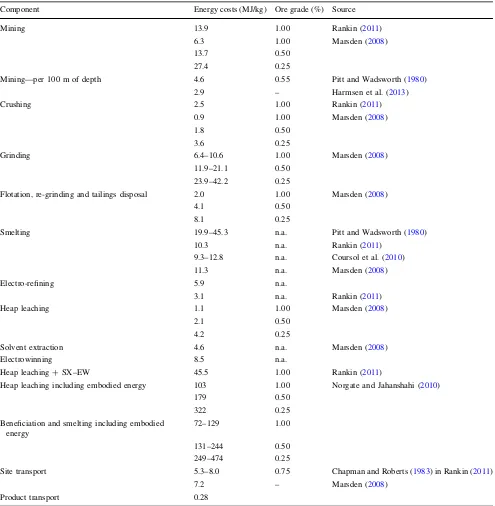
size was established at 129, 244 and 474 MJ/kg. The large increase can be explained because substantially more operational inputs such as steel balls in mills and flotation chemicals are used as grinding sizes get smaller; as such, Table 1 Summary of copper energy input cost values from the existing literature
Component Energy costs (MJ/kg) Ore grade (%) Source
Mining 13.9 1.00 Rankin (2011)
6.3 1.00 Marsden (2008)
13.7 0.50
27.4 0.25
Mining—per 100 m of depth 4.6 0.55 Pitt and Wadsworth (1980)
2.9 – Harmsen et al. (2013)
Crushing 2.5 1.00 Rankin (2011)
0.9 1.00 Marsden (2008)
1.8 0.50
3.6 0.25
Grinding 6.4–10.6 1.00 Marsden (2008)
11.9–21.1 0.50
23.9–42.2 0.25
Flotation, re-grinding and tailings disposal 2.0 1.00 Marsden (2008)
4.1 0.50
8.1 0.25
Smelting 19.9–45.3 n.a. Pitt and Wadsworth (1980)
10.3 n.a. Rankin (2011)
9.3–12.8 n.a. Coursol et al. (2010)
11.3 n.a. Marsden (2008)
Electro-refining 5.9 n.a.
3.1 n.a. Rankin (2011)
Heap leaching 1.1 1.00 Marsden (2008)
2.1 0.50
4.2 0.25
Solvent extraction 4.6 n.a. Marsden (2008)
Electrowinning 8.5 n.a.
Heap leaching?SX–EW 45.5 1.00 Rankin (2011)
Heap leaching including embodied energy 103 1.00 Norgate and Jahanshahi (2010)
179 0.50
322 0.25
Beneficiation and smelting including embodied energy
72–129 1.00
131–244 0.50
249–474 0.25
Site transport 5.3–8.0 0.75 Chapman and Roberts (1983) in Rankin (2011)
7.2 – Marsden (2008)
the embodied energy also grows. The study also evaluated heap leaching direct and embodied energy inputs at 103, 179 and 332 MJ/kg, respectively.
Finally, depending on the processing setup substantial transportation costs will be required if the distance from the beneficiation to the smelting & refining site are sub-stantial. Transport cost for Freeport-McMoRan operations with separated locations was evaluated by Marsden (2008) at 7.2 MJ/kg, versus negligible for close proximity opera-tions. Additional transport costs to bring the copper cath-odes to market were evaluated at 0.28 MJ/kg by Marsden (2008). The evaluation in Rankin (2011) yields a 40–60 MJ cost per ton of rock moved between site oper-ations based on values in Chapman and Roberts (1983), which translates into 5.3–8.0 MJ cost per kg of copper at a 0.75% ore grade.
Methodologies and Data Input
Parsimonious Energy Cost Relation
The effects of ore grades and mining depth are combined to develop a parsimonious relation to estimate mining and beneficiation energy costs with as few variables as possi-ble. The analysis is carried out from per metric ton of metal produced perspective. As a starting point the relation specified in Page and Creasey (1975) is taken, where the amount of energy E, required to mine and concentrate a mineral is reciprocally dependent on a specific head grade, G, weighed byb, i.e., the energy costs to process a metric ton of copper bearing ore. The head grade values are inserted in numerical form. Their relation is specified as:
E¼aþb=G ð1Þ
where E is the processing (by extraction and milling/ flotation or leaching) energy usage in MJ per kg of copper concentrate at 30%? purity or copper in pregnant leach solution. The fixed energy cost parameterb is divided by an ore grade variableGin percentage of copper per mass of ore extracted, so as to capture changes in energy costs. The parametera is added as the fixed minimum extraction and processing energy costs.
Equation (1) expresses roughly that ore grades halve the effort to extract doubles and that this scales linearly. It could also be when ore grades decline energy costs will rise at an accelerating rate. This behavior obeys a power law and can be specified as:
E¼gG e ð2Þ
where energy usage for obtaining concentrate copper in MJ per kg is based on the ore grade G to the power of a negative parametere, and multiplied by a parameterg, so
as to capture accelerating growth in energy costs due to lower ore grades.
A third relation is simplified from the model in Pitt and Wadsworth (1980) as the transport energy cost usageE in MJ per kg of copper moved, being dependent on the ver-tical distanceDfrom the concentrator at the surface to the deepest mine point weighed by its energy costs. The parameterccaptures the effects of depth per meter.
E¼aþcD ð3Þ
Again the parameter a is added for the fixed minimum extraction and concentrating energy costs. In the literature, commonly depth is incorporated separately from ore grades (Rankin2011; Harmsen et al.2013), which implies that ore grades have limited influence on the degree of rock that has to be lifted, or at least under present circumstances. This assumption is used to functionally add Eqs. (1) and (3) resulting in Eq. (4) and the addition of Eqs. (2) and (3) resulting in Eq. (5). The two Eqs. (4) and (5) enable a combined ore grade and depth evaluation.
E¼aþcDþb=G ð4Þ
E¼aþcDþgG e ð5Þ
The effects of depthDplausibly interact with ore gradesG, since a lower ore grade implies that more copper bearing rock has to be lifted to a milling or leaching facility. Based on this logic, both the first and third equations are func-tionally combined, by substitution of parameter b and parameter g in the right-hand side of Eqs. (1) and (2), respectively, with the right-hand side cD of Eq. (3), which results in Eqs. (6) and (7) with interaction between depth and ore grade effects on energy costs:
E¼aþcD=G ð6Þ
E¼aþcDG e ð7Þ
with extraction energy usage E in MJ per kg concentrate copper based on the depthDof mining and ore gradeGin percentage of copper per mass of ore. The parametercnow captures the joint effects of both depth and ore grade dif-ferences per mine. The equations can be used for total energy inputs or to assert the effect of diesel and electricity individually, in relation to ore grades and depth.
By-Products Evaluation
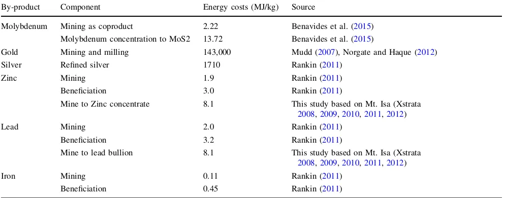
magnetite. Annual output quantities for these by-products were established either directly from mining company reports or if unavailable based on ore by-product content. Subsequently, output quantities were multiplied by the literature values for energy cost per metric ton included in Table2. Finally, the by-product energy cost was subtracted for the copper content energy costs. The calculation for by-products is included in the data spreadsheet supplement B to this paper. As an example of the procedure in the spreadsheet, alongside copper in 2011 the Los Pelambres mine in Chile produced 57.25 metric ton of silver, 1.13 metric ton of gold and 9900 metric ton of molybdenum. The energy inputs estimated for these by-products were 98, 161 and 158 TJ for silver, gold and molybdenum, respec-tively. The total sum of 417 TJ was subtracted from total energy inputs of 7047 TJ to establish the net-of-by-product energy cost per metric ton of copper. The calculation was only carried out for total energy since by-product per metric ton energy values were primarily found in the lit-erature on a sum of energy basis.
Statistical Testing Procedure
The parsimonious relations in the previous section are assessed statistically using a large dataset for copper mines based on the energy costs of mining, concentrating and smelting, the head grade of the extracted ore at the milling stage and the depth of the mine. Data were separated in the analysis between surface mines and underground mines, so as to examine whether there are differences between main mining types. Each of the Eqs. (1), (2), (3) and (4) was tested as outlined in the previous section. The analysis was carried out using linear and nonlinear regression in the R statistics package. Prior to carrying out the tests, firstly an
evaluation of potential outliers was carried out, and sec-ondly, the normality of the data was tested using a Sha-piro–Wilk test and a Q–Q plot analysis, as described in ‘‘Results’’ section. Results are reported and evaluated in ‘‘Data inputs’’ section based on whether a null hypothesis of a significant relation is accepted or rejected, the standard error of residuals, a R2 goodness-of-fit measure for Eqs. (1), (3), (4), (6), and pseudo-R2 for the nonlinear Eqs. (2), (5) and (7), and a correlation between predicted results and sample data values.
Data Inputs
Energy and Mines
Fuel, electricity and all input energy data were gathered for 28 copper mining operations operated by companies Anglo-American, Antofagasta, BHP Billiton, CODELCO, China Molybdenum, Lundin Mining, Oz Minerals, Rio Tinto, Sterlite, Grupo Mexico Southern Copper Company, Vedanta and Glencore Xstrata. The observations originated from nine countries, Australia, Chile, Mexico, Peru, Por-tugal, South Africa, the USA and Zambia. In total, 194 datasets were gathered spanning from 2003 to 2015, including the attributes mine name, mine-type, country, operator, year, processing route, heap grade, mine-depth, energy input, by-products. In case a heap grade value for mined material was not available, the average reserve ore grade value was taken.
The data were organized to enable distinction between four data attributes and their variants for the statistical analysis or pre-/postprocessing:
Table 2 By-product energy cost values used from the existing literature
By-product Component Energy costs (MJ/kg) Source
Molybdenum Mining as coproduct 2.22 Benavides et al. (2015)
Molybdenum concentration to MoS2 13.72 Benavides et al. (2015)
Gold Mining and milling 143,000 Mudd (2007), Norgate and Haque (2012)
Silver Refined silver 1710 Rankin (2011)
Zinc Mining 1.9 Rankin (2011)
Beneficiation 3.0 Rankin (2011)
Mine to Zinc concentrate 8.1 This study based on Mt. Isa (Xstrata 2008,2009,2010,2011,2012)
Lead Mining 2.0 Rankin (2011)
Beneficiation 3.2 Rankin (2011)
Mine to lead bullion 8.1 This study based on Mt. Isa (Xstrata
2008,2009,2010,2011,2012)
Iron Mining 0.11 Rankin (2011)
• Mine-type, surface mines (open-pit, open-cut), under-ground mines (block-caving, sub-level stopping) and sites covering both.
• Deposit type, porphyry, volcanogenic massive sulfide, iron oxide copper gold, metamorphic, stratabound, exotic and carbonatite-hosted magnetite–copper sulfide.
• Processing routes, including mines with metal-lurgy to concentrate (milling and flotation), pyro-metallurgy to cathode, hydropyro-metallurgy (leaching and SX–EW) and mine-sites with both pyro- and hydromet-allurgy routes.
• Produced outputs, mined copper processed,
concen-trate produced, copper leached, concentrate and leachate processed, anodes, cathodes and rods produced.
After collection, the energy, output and by-products data were translated to a MJ per kg of copper basis by the end-product point of the mine and gross- and net-of-by-end-product. The data were taken from sustainable development reports, company quarterly operational reports, global reporting initiative statements (GRI) (GRI 2013a) and annual reports. In supplement A to this paper, a complete bibliography of the 310 used reports is included organized per company. The entire dataset is given in supplement B.
Mine-Depth
The height difference between the surface leaching or concentrator facility and the deepest point of the mine-site was estimated to obtain mine-depth. In case of underground mines, the value for the depth of the main mine shaft or mining to transport level was taken. Data were obtained from a mining literature screening for 24 out of 28
mine-sites and GIS contour maps from digital elevation model (DEM) satellite data for 25 mine-sites. In case multiple values were available, from either the literature or satellite data, the data were incorporated in order of the ranking (1) mine schematics with elevation values, (2) mining industry peer-review literature, (3) official company sources, (4) satellite data, (5) other third-party data. The contour maps were generated from one arc-second (30.87-m interval) ASTER GDEM v2 data (NASA2011). The vertical accu-racy of the dataset has been compared against 18,000 geodetic control points and has been found to be within 17-m accuracy at a 95% confidence level (Tachikawa et al. 2011). To contrast these data, Google Earth utilizes older three arc-second (90-m interval) SRTM v2 data for eleva-tion. The obtained GDEM v2 tiff files were translated into contour maps using QGIS software from which the height difference was visually observed, as shown in Fig.1for the Bingham Canyon and Chuquicamata copper mines. The literature mine-depth bibliography and generated contour maps for each mine are added as supplement C to this paper for reference purposes.
Preprocessing
data adjustment). The values for solvent extraction and electrowinning were taken from (Marsden2008) at 4.6 and 8.5 MJ/kg, respectively.
The dataset was evaluated for outliers, based on visual inspection of the independent variables head grade and depth to the dependent variable energy costs. The data from the Konkola Copper Mines in Zambia were found to be an extreme outlier, relative to the other data points, and removed from the datasets. The rationale for removal was the high energy costs, despite a 3% head grade underground mine, to be due to high quantities of water pumped to maintain a dry environment. Pumping vol-umes are estimated at 400.000 m3/day, or 365 to 440 m3/metric ton of copper produced. In contrast, water pumping requirements for other copper mines are a factor ten lower, such as the 1%?head grade Mount Lyell mine
operated by Copper Mines of Tasmania, with 27–35 m3 water pumped per metric ton copper (Vedanta Resources 2010).
After the removal of outliers, additional testing was carried to assess whether the error values of the linear equations were normally distributed, so as to assure validity of the statistical methods. A two-step approach was taken, with as a first step a visual means using a QQ plot wherein the standardized residuals from the empirical data were ranked against the standard normal residuals (Walpole et al.1998). The data were found not to exhibit a normal distribution in all cases and it was chosen to transform the linear Eqs. (1), (3), (4) and (6) into a log-linear model. The transformed data were found to pass normality, as shown for the 191 value dataset in Fig.2 and Table3.
Fig. 2 Assessment of normality of the datasets using a QQ plot procedure based on
standardized residuals of Eqs. (1), (3), (4) and (6)
Table 3 Results of Shapiro–
Wilk analysis of normality Shapiro–Wilk test on standardized residuals Log-linear equations
(1) (3) (4) (6)
Test statisticsW 0.915 0.935 0.898 0.949
Results
Descriptive Data: Ore Grade and Depth
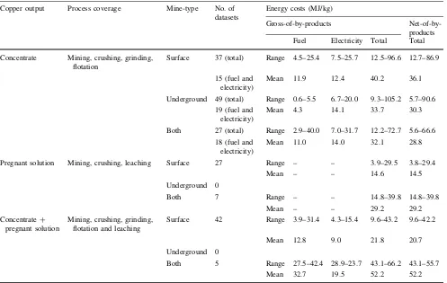
The mine energy data are summarized in Table4 for obtaining a copper concentrate via pyro-metallurgy, a pregnant solution via hydrometallurgy, or mines producing both. The values net-of-by-products from mining to pro-duct can be summarized as:
• The energy costs forcopper concentrate from surface mines were established in a range from 12.7 to 86.9 with a mean of 36.1 MJ/kg. The highest cost values in the range came from the Porphyry deposit Bingham Canyon open-pit mine in the USA with a depth estimate of 900 m and ore grade average of 0.56% across the dataset period. In contrast, the lowest cost values were derived from the Porphyry deposit Los Pelambres open-pit mine in Chile with a depth estimate of 300 m and a 0.74% ore grade average.
• The energy costs for copper concentrate from
underground mines were established in a range from 5.7 to 90.6 with a mean of 30.3 MJ/kg. The highest cost
values in the range came from the carbonatite-hosted magnetite–copper sulfide deposit Palabora block-cave mine in the USA with a depth estimate of 800–2100 m and ore grade average of 0.66% across the dataset period. In contrast, the lowest cost values were derived from the volcanogenic massive sulfide deposit Mount Lyell sub-level caving mine in Australia which has a depth estimate of 1000 m and a 1.21% ore grade average.
• The energy costs for leachingpregnant solution from
surface mineswere established in a range from 3.8 to 29.4 with a mean of 14.5 MJ/kg. The highest cost values in the range came from the porphyry deposit Cerro Colorado open-cut mine in Chile with a depth estimate of 230 m and ore grade average of 0.74% across the dataset period. In contrast, the lowest cost values were derived from the porphyry deposit Spence open-cut mine in Chile with a depth estimate of 80 m and a 1.3% ore grade average.
The values were also established for fuel and electricity cost components. First, a significant difference can be observed between surface and underground mines in case
Table 4 Results from mine energy datasets including preprocessing
Copper output Process coverage Mine-type No. of datasets
Energy costs (MJ/kg)
Gross-of-by-products
Net-of-by-products Fuel Electricity Total Total
Concentrate Mining, crushing, grinding, flotation
Surface 37 (total) Range 4.5–25.4 7.5–25.7 12.5–96.6 12.7–86.9
15 (fuel and electricity)
Mean 11.9 12.4 40.2 36.1
Underground 49 (total) Range 0.6–5.5 6.7–20.0 9.3–105.2 5.7–90.6
19 (fuel and electricity)
Mean 4.3 14.1 33.7 30.3
Both 27 (total) Range 2.9–40.0 7.0–31.7 12.2–72.7 5.6–66.6
18 (fuel and electricity)
Mean 11.0 14.0 32.1 28.8
Pregnant solution Mining, crushing, leaching Surface 27 Range – – 3.9–29.5 3.8–29.4
Mean – – 14.6 14.5
Underground 0
Both 7 Range – – 14.8–39.8 14.8–39.8
Mean – – 29.2 29.2
Concentrate? pregnant solution
Mining, crushing, grinding, flotation and leaching
Surface 42 Range 3.9–31.4 4.3–15.4 9.6–43.2 9.6–42.2
Mean 12.8 9.0 21.8 20.7
Underground 0
Both 5 Range 27.5–42.4 28.9–23.7 43.1–66.2 43.1–55.7
Mean 32.7 19.5 52.2 52.2
of pyro-metallurgical processing as the latter have much lower fuel inputs. Second, the fuel input difference found between pyro- and hydrometallurgical mines was not found to be substantial, but the electricity input into hydromet-allurgical mines was lower.
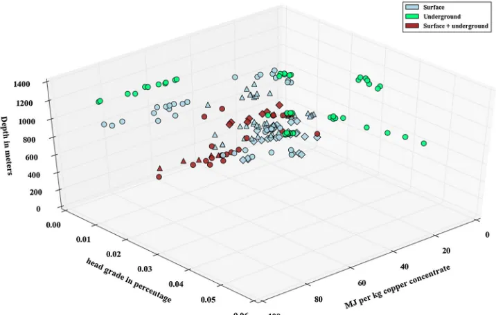
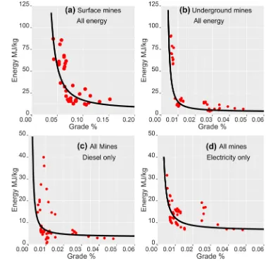
The values net-of-by-products are also displayed against head grades and depth the three-dimensional plot in Fig.3. A hyperbolic shape versus head grade values can be observed visually, where energy costs go up rapidly below a 1% pro-cessed head grade, based on observed head grades with a 0.22–4.8% range with a 1.03% mean value. The effect of depth appears less pronounced as there are both mines with a depth of 700?m with low energy costs below 20 MJ/kg and mines with a 700?m depth with 50?MJ/kg energy values. However, the mines with low energy costs all have head grades above 1% and vice versa. Moreover, the effect of depth appears to be absent fully for mines with only leaching operations for processing. The depth of mines was found to range between 50 and 1200 m with a mean of 530 m.
The data for fuel and electricity for produced concentrate from pyro-metallurgy are plotted against head grades and depth and are shown in Fig.4. The first observation is that electricity usage in MJ/kg of concentrate for mines at 200? depth levels is larger than diesel use, while the opposite is the case for mines at lower depths. Second, the hyperbolic shape observed earlier can also be discerned on a separate basis for diesel and electricity for copper concentrate.
Statistical Analysis Depth and Ore Grade Effects
The seven equations as per Sect. 2 were tested for eight different datasets varying by surface or underground mines,
and by milling/flotation or heap leaching, as well as anal-yses for total energy or diesel and electricity both sepa-rately. The diesel and electricity tests were only carried out for concentrate and for mixed concentrate?PLS mines, since in case of underground/surface separation too few data points are available for an adequate statistical test. The linear Eqs. (1), (2), (4) and (6) were log-linearly adjusted as described in Sect. 2.
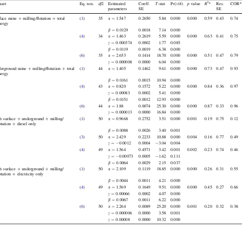
The full results are added in supplementary materials D with the results of the best fitted Eq. (4) shown in Table5 for underground and surface mines, as well as in visual form in Fig.5. The results can be summarized as follows:
• All data, with the complete 191 point dataset all
equations provided a significant result except Eq. (7). The best fit was found for Eq. (5) which provided anR2 of 0.37 and a correlation of 61% with predicted results.
• Surface and underground mines with
milling/flota-tion processing Eqs. (1), (3), (4) and (6) were all significantly below a 5% significance threshold, with the best result being found for Eqs. (4) and (6). The surface mine dataset yielded a R2 of 0.63 and a correlation of 75% with predicted data for Eq. (4), and for underground mines aR2of 0.84 and a correlation of 97%.
• Mines with leaching onlyyielded no significant result
for any of the equations for neither ore grade nor depth. The depth variation ranges from 50 to 600 m in the dataset, and the ore grade variation ranges between 0.3 and 1.65%.
• Diesel and electricity with milling/flotation
process-ingshowed significant results for diesel with Eqs. (1), (3), (4) and for electricity Eqs. (1), (4) and (6). The best Fig. 3 Three-dimensional plot
of energy costs plotted against mine-depth and ore grade data with values for open-pit mines (blue), underground mines (green) and mine-sites with both (red) as well as distinction by processing route pyro-metallurgy (circles),
results were found with Eq. (4) with anR2for diesel of 0.23 plus a correlation with predicted values of 46% and an R2 for electricity of 0.45 with correlation of 66%.
• Mines with both milling/flotation and leaching
operationsshowed no significant results for electricity and for diesel significant results for Eqs. (1), (3) and (4). The best result was Eq. (4) with anR2of 0.43 and a correlation of 53% with predicted values.
The general observation from the results is that com-bined depth and ore grade models, for mines with milling/ flotation mines, performed better over models with only head grades or depth, showing the value of added infor-mation. In case of surface and underground mines with milling/flotation, Eqs. (4) and (6) with combined depth and ore grades have the lowest residual standard error and highest R2 values for all three datasets. However, the parameter for depth for the diesel case is negative render-ing its influence opposite as expected, although it is posi-tive for electricity The ore grade only Eq. (1) is the only one found suitable for diesel, albeit with low explanatory power.
The key difference between Eqs. (4) and (6) is the lowest standard error of coefficients for Eq. (4) combined with better predictive value for electricity usage. This warrants the first conclusion: Statistically Eq. (4) is the best model for mines with milling/flotation. On the basis of this, an ore grade of 0.5, 0.4 and 0.3% at 300 m of depth results in an energy cost of 60, 127 and 447 MJ/kg for under-ground mines, and 52, 95 and 255 MJ/kg for surface mines, respectively. The second conclusion is that no significant results are found for heap leaching operations where head
grade and depth appear to have no direct relation with energy use. The third conclusion is that depth only had a substantial effect on electricity use for mines with milling and flotation operations, with limited influence on diesel usage. The effect is potentially due to the higher electricity needs in underground mining for purposes of haulage by rail and conveyor belts as opposed to trucks. The fourth conclusion is that ore grades have a more significant effect on energy cost for underground mines than surface mines.
Discussion
Dataset Uncertainty
The datasets used to evaluate the ore grades and depth impacts were taken from over 14 companies over a decadal time span. Although these analyses are carried out by different teams, the energy data values taken from company sustainability reports are structured using the common global reporting initiative (GRI) for the mining industry (GRI2013a). For example, the GRI standardises the evaluation of energy data into direct within organization and indirect purchased energy consumed by primary energy source and technology type (GRI2013b). The second main data uncertainty lies in evaluated mine-depth values, which were taken from various literature sources and 1 arc-second generated mine contour map observations. For 14 out of 20 mines both estimates where available, and it was found that in all 14 cases the depth difference between esti-mates was within 100 m. The challenge of using this proxy lies in that mine-designs vary substantially especially for underground mines, where mined ore may be lifted down the mine instead of up, for example, in case of El Teniente in Fig. 4 Three-dimensional plot
Chile, due to its location high above in the mountains. Also mine-depth changes on a gradual basis, whereas in most cases a single depth value was established for multiple years. The other assumption of the height difference is also an over-simplification as mining takes place at various levels in the mine. A rigorous analysis would establish the exact depth/ height, transport distances and transport process (conveyor belt, truck hauling), and how it changes per year, but this was not feasible in the absence of sufficiently detailed data. Nonetheless, the values for mine-depth do provide for an attempt to evaluate the depth effect on mine-types and pro-cessing routes.
Validity of Methodology
The main challenge to the statistical relationship can in view of the authors be made on the extent to which the model relations will remain similar, since they are groun-ded in current technologies, mine-design and efficiency. The mining industry is well aware of the key role of energy in mining and is involved in significant efforts to reduce these costs where possible. For example, the potential number of meters drilled per hour in underground mining increased from 275 to 450 m between 2000 and 2005 due to an improved design of the Atlas Copco rocket boomer Table 5 Selection of results for ore grade- and depth-related energy cost models
Dataset Eq. nos. df2 Estimated
parameters
Coeff. SE
T-stat Pr([|t|) pvalue R2* Res.
SE
COR**
Surface mine?milling/flotation?total energy
(1) 35 a¼1:547 0.2650 5.84 0.000 0.000 0.59 0.43 0.74
b¼0:0129 0.0018 7.14 0.000
(4) 34 a¼1:463 0.2619 5.59 0.000 0.000 0.63 0.41 0.75
c¼0:000374 0.0002 1.77 0.085 b¼0:0119 0.0019 6.38 0.000
(6) 35 a¼2:653 0.1414 18.70 0.000 0.000 0.51 0.47 0.79 c¼0:000008 0.0000 6.04 0.000
Underground mine?milling/flotation?total energy
(1) 44 a¼1:405 0.1462 9.61 0.000 0.000 0.73 0.47 0.93
b¼0:0161 0.0015 10.94 0.000
(4) 43 a¼0:820 0.1572 5.22 0.000 0.000 0.84 0.36 0.97
c¼0:00083 0.0002 5.41 0.000 b¼0:0151 0.0012 12.93 0.000
(6) 44 a¼1:88 0.0074 25.30 0.000 0.000 0.87 0.33 0.96 c¼0:000013 0.0000 16.84 0.000
Both surface?underground?milling/ flotation?diesel only
(1) 50 a¼0:9668 0.2752 3.51 0.000 0.001 0.19 0.75 0.12
b¼0:0088 0.0026 3.40 0.001
(3) 50 a¼2:429 0.2233 10.88 0.000 0.004 0.16 0.77 0.49
c¼ 0:0012 0.0004 -3.04 0.004
(4) 49 a¼1:564 0.4571 3.42 0.001 0.002 0.23 0.74 0.46
c¼ 0:00073 0.0005 -1.62 0.111 b¼0:0064 0.0029 2.15 0.037 Both surface?underground?milling/
flotation?electricity only
(1) 50 a¼2:109 0.1119 18.85 0.000 0.000 0.26 0.31 0.55
b¼0:0044 0.0011 4.21 0.000
(4) 49 a¼1:569 0.1649 9.51 0.000 0.000 0.45 0.27 0.66
c¼0:00066 0.0002 4.07 0.000 b¼0:0067 0.0011 6.22 0.000
(6) 50 a¼2:264 0.0089 25.20 0.000 0.001 0.20 0.32 0.38
c¼0:000006 0.0000 3.58 0.001 c¼0:00008 0.0000 10.32 0.000
* Pseudo-R2is listed using pseudo-R2=1-SSE/SSTOTAL for nonlinear equations
drill machine (Ericcson2014). And the use of diesel rail-way haulage is increasingly replaced by electric haulage and belt conveying in underground mining, which has the advantage of reducing energy-intensive underground ven-tilation needs (Salt and Mears2006; International Mining 2009). While the technological developments and their implications are well understood in the mining industry, they have to the awareness of the author’s not yet been quantified in a precise manner in terms of their historic influence on energy costs. A more precise evaluation of the historic progression in energy efficiency of different min-ing processes in quantified terms would enhance the meaningfulness of future projection, by substantiation of the validity of relations in the long term of several decades, or lack thereof.
The second key issues with validity lie in the focus on a macro-level of analysis, which limits the ability to dig into the rationale for the results to corroborate the statistical findings, such as mine-designs and specific physical factors at the rock and mineral level for energy costs. These can include among others mine to concentrator or leaching
heap distance, mine-water processing route, mine slopes, the particle size of the initial ore, the grinding size after crushing, cutoff grade decisions, the hardness of the ore, the presence of refractory ore and impurities (Hustrulid et al.2000). While general observations can be made, such as that reliance on electricity increases with deeper mines, a more detailed evaluation would be add to the explanatory power of the found relations (or lack thereof) such as using grind-size effect equations (Morrell2004,2010). The level of detail is in view of the authors outside of the scope of this macro-level analysis, as it would warrant a different methodology such as in the form of a physical life cycle mine-simulation model using difference–differential equations and annual mine-planning plus operational decisions.
Interpretation of Results
The results need to be viewed within the energy boundaries of the analysis, which included direct and indirect energy, and excluded energy use associated with materials used in Fig. 5 Data points and Eq. (4)
extraction and processing. For example, the steel balls used in milling and the chemicals used in flotation and heap leaching. The lack of an observed relation for leaching to ore grades may be because a substantial portion of the energy comes from material costs due to the chemical nature of the process, as established by Norgate and Jahanshahi (2010) in their life cycle analysis. Another boundary aspect relates to the way electricity is incorpo-rated as final energy, since for macro-level global energy evaluations a comparison at primary energy levels for fossil fuel to electricity conversions is necessary.
In the statistical analysis itself, datasets were not por-tioned up into mineral deposit types because of too limited groupings for statistical purposes. However, mineral geol-ogy can affect energy costs when looking at individual mines. The Cu-stratabound deposit in which the Michilla mine in Chile sits, for instance, has narrow mineral layers which could be of significance in explaining its higher energy costs relative to other heap leaching-based mines in the dataset. Similarly, the sub-level stopping underground mining methods used for the Candelaria mine and Promi-nent Hill Ankata underground mine may provide for energy cost disadvantages over block-caving mines such as El Teniente, Rio Blanco and Northparkes (Taggart et al. 2012). Other mine-specific factors can include water treatment and pumping needs due to increasing use of desalination such as increasingly the case in copper mines in Chile to several kilometers high, which can easily double water energy costs from conventional water treat-ment (Zhou and Tol 2005; Jamasmie 2014). Since such mine-specific factors are not taken into account, the results cannot be directly interpreted for individual mines, but should only be interpreted at the general level of copper mining and processing using flotation/milling and heap leaching, with distinctions between surface and under-ground as well as diesel and electricity usage.
Implications of Results
The average ore grade of a mining project today is estimated around 0.76% which for a milling-/flotation-based mine using Eq. (4) translates into an energy cost of 24 and 24.5 MJ/kg at 450 m depths for underground and surface mines, respec-tively. This translates based on the 19.9 million metric tons of copper produced to an energy cost of around 0.84 ExaJoules (about 0.14% of global 550 ExaJoules energy use), when assuming an additional 18 MJ for smelting/refining and transport (Siirola2014). The lowest ore grade mine-sites in the dataset include the El Salvador (surface?underground), Bingham Canyon (surface) and Palabora (underground) mines which have ore grades close to 0.5% in recent years, mine-depths of 150, 900 and 1200 m, and average 2010–2013 energy costs of 47, 81 and 93 MJ/kg, respectively. If average
ore grades increase to the levels of these mines, energy costs of mining from milling/flotation operations could triple globally. In contrast, the energy costs of scrap copper recycling has been established at 6.3 and 18 MJ/kg (Grimes et al.2008; Ashby 2009). However, the referenced studies do not include trans-port energy requirements to bring scrap copper to the pro-cessing plant, and a more complete comparative study of the benefits of recycling versus mining would be a promising avenue of further research.
The upstream cost impacts in copper products can be illustrated by the copper content in a kilometer of low-voltage 0.6/1 kV copper cables which is used for underground cabling at street level in local electricity distribution grids in many countries. In the UK, the standard cable is a 3-phase 35 mm2 copper cable, which contains 1750 kg of copper per km (Eurocable Group2011; Scottish Power2012). The average price of pure copper cathode was 3.1 USD per kg in 2014 (IWG2016). A cost estimate for 0.6/1 kV cables from an Indian manufacturing company in 2014 was retrieved at 32,800 USD per kilometer (LC International2014). There-fore, the approximate copper content cost proportion is 20% in a low-voltage cable at retail. Based on data from the Grasberg and Escondida mines, the first and third largest in the world with ore grades above 1.2 and 0.7%, respectively, the energy costs for cathode copper were found to fluctuate between 10 and 15% before 2003, and a 15–30% share between 2007 and 2009 for these two mines (Minera Escondida 2008,2009,2010; World Mine Cost Data Exchange2010a,b). The energy cost of copper wire therefore fell within a 2–6% range in recent times, which makes energy cost increase impacts on the final product limited yet still relevant when considering high energy prices scenarios. A tripling of energy costs would result in a 4–12% increase in product prices based on the analysis above. A rise appears to be relatively insignificant, since it is far outweighed by overall energy price fluctuations and their impacts on copper energy mining costs. An integrated analysis of copper energy costs and energy prices scenarios is therefore necessary in the examination of energy cost effects on financial costs of copper products.
sources. In the foreseeable future, the ability for a copper project to be affordable is therefore highly related to the regional power source and its costs, unless an affordable storage solution for continuous industrial operations emerges which at present is unlikely.
Conclusions
This study concludes with four summarizing observations drawn from the results and discussion:
• The best explanation for energy costs of mines with
milling/flotation processing, for both surface and underground mines, was found in an equation with an interactive effect between depth and ore grades, as opposed to taking these factors as independent.
• The evaluation for mines with milling/flotation found
that ore grades had a significant impact on both diesel and electricity use, while in case of depth only electricity was substantial influenced with only limited to no contribution from depth variation. Also it found that ore grade and depth effects are more significant for underground than surface mines.
• Neither ore grades nor depth had a significant influence
on energy use for mines that solely utilized leaching operations for extracted ore.
• The impacts on energy costs from mine extraction to
concentrate copper from milling/flotation based on the validated log-linear Eq. (4) were found to accelerate significantly at a 0.5% or lower ore grade (e.g.,[55 and
67 MJ/kg for surface and underground, respectively, at 450 m of depth), which can be interpreted as a biophys-ical barrier at present technologies below which copper mining extraction using milling/flotation becomes increasingly challenging from a cost perspective.
• The depth impacts on electricity for mines with milling/
flotation were evaluated from the statistically validated log-linear equation at a 7% increase in copper mining and concentrating electricity costs per 100 m of mine-depth under present technologies.
Open Access This article is distributed under the terms of the Creative Commons Attribution 4.0 International License (http://creative commons.org/licenses/by/4.0/), which permits unrestricted use, distri-bution, and reproduction in any medium, provided you give appropriate credit to the original author(s) and the source, provide a link to the Creative Commons license, and indicate if changes were made.
References
Ashby MF (2009) Materials and the environment: eco-informed material choice, 1st edn. Butterworth-Heinemann, Oxford
Bardi U (2013) The mineral question: how energy and technology will determine the future of mining. Front Energy Res 1:9. doi:10.3389/fenrg.2013.00009
Barnett HJ (1979) Scarcity and growth revisited. In: Smith KV (ed) Scarcity and growth reconsidered, 1st edn. John Hopkins University Press, Baltimore
Benavides PT, Dai Q, Sullivan J et al (2015) Material and energy flows associated with select metals in GREET2. Argonne National Laboratory/ESD-15/11
Borgmann M (2016) Dubai shatters all records for cost of solar with earth’s largest solar power plant. Apricum, Berlin
Brininstool M (2016) USGS mineral commodity summaries, January 2016: copper. US Geological Survey, VA, pp 54–55
Chapman PF, Roberts F (1983) Metal resources and energy. Butterworth-Heinemann, London, 238 pp.http://www.sciencedir ect.com/science/book/9780408108010
CODELCO (2015) CODELCO update April 2015, p 19
Coursol P, Mackey PJ, Diaz C (2010) Energy consumption in copper sulphide smelting. Proceedings of Copper 2010, Vol. 2— Pyrometallurgy I. GDMB, Clausthal-Zellerfeld, pp 649–668 Crowson P (2003) Mine size and the structure of costs. Resour Policy
29:15–36. doi:10.1016/j.resourpol.2004.04.002
Crowson P (2012) Some observations on copper yields and ore grades. Resour Policy 37:59–72. doi:10.1016/j.resourpol.2011. 12.004
Davenport W, King M, Schlesinger M, Biswas A (2002) Extractive metallurgy of copper, 4th edn. Pergamon, Oxford
Emsley J (2001) Nature’s building blocks: an A–Z guide to the elements, 1st edn. Oxford University Press, New York Ericcson M (2014) Supply and demand: innovation drivers in the
minerals industry. In: Anderson CG, Dunne RC, Urie JL (eds) Mineral processing and extractive metallurgy, 1st edn. Society for Mining, Metallurgy, and Exploration, Englewood, pp 3–13 Eurocable Group (2011) Product catalog. Jakovlje, Croatia, pp 24–25.
http://www.eurocable-group.com/wp-content/uploads/2013/07/ eurocable_group_-_product_catalog_2011.pdf. Accessed 25 Feb 2016
Fuerstenau MC, Jameson GJ, Yoon R-H (2007) Froth flotation: a century of innovation. Society for Mining, Metallurgy, and Exploration, Littleton
GRI (2013a) G4 sector disclosures: mining and metals. Global Reporting Initiative, Amsterdam
GRI (2013b) G4 sustainability reporting guidelines—part 2: imple-mentation manual. Global Reporting Initiative, Amsterdam Grimes S, Donaldson J, Gomez GC (2008) Report on the
environ-mental benefits of recycling. Bureau of International Recycling, Brussels, 54 pp
Hall CAS, Cleveland CJ, Kaufmann R (1986) Energy and resource quality: the ecology of the economic process, 1st edn. Wiley, New York
Harmsen JHM, Roes AL, Patel MK (2013) The impact of copper scarcity on the efficiency of 2050 global renewable energy scenarios. Energy 50:62–73. doi:10.1016/j.energy.2012.12.006 Hustrulid WA, McCarter MK, Van Zyl DJA (2000) Slope stability in
surface mining, 1st edn. Society for Mining, Metallurgy, and Exploration, Littleton
International Mining (2009) The El Teniente conundrum. InfoMine, pp 62–63
IWG (2016) Omega—Camden copper base price. http://www. iwgcopper.com/price-history?year=2015. Accessed 25 Feb 2016 Jamasmie C (2014) Chile set to make mining desalination mandatory. http://www.mining.com/chile-set-to-make-mining-desalination-mandatory-57150/. Accessed 18 July 2016
Layton M, Fu Y, Currie J (2015) Metal detector: China copper to aluminium substitution set to accelerate. Goldman Sachs Global Investment Research, New York
LC International (2014) Price list effective from 1st July 2014.http:// www.lccables.com/armd.html. Accessed 26 Feb 2016
Marsden JO (2008) Energy efficiency and copper hydrometallurgy. In: Young CA, Taylor PR, Anderson CG, Choi Y (eds) Hydrometallurgy 2000: proceedings of the sixth international symposium. Society for Mining, Metallurgy, and Exploration, Colorado
Metso (2010) Basics in minerals processing. Metso Corporation, Helsinki, 354 pp.http://bit.ly/2g8JADl. Accessed 11 July 2016 Minera Escondida (2008) Escondida financial statements 2007.
Antofagasta
Minera Escondida (2009) Financial statements 2008. Antofagasta Minera Escondida (2010) Estados Financieros 2009. Antofagasta Morrell S (2004) An alternative energy-size relationship to that
proposed by Bond for the design and optimisation of grinding circuits. Int J Miner Process 74:133–141. doi:10.1016/j.minpro. 2003.10.002
Morrell S (2009) Predicting the overall specific energy requirement of crushing, high pressure grinding roll and tumbling mill circuits. Miner Eng 22:544–549. doi:10.1016/j.mineng.2009.01.005 Morrell S (2010) Predicting the specific energy required for size
reduction of relatively coarse feeds in conventional crushers and high pressure grinding rolls. Miner Eng 23:151–153. doi:10. 1016/j.mineng.2009.10.003
Mudd GM (2007) An analysis of historic production trends in Australian base metal mining. Ore Geol Rev 32(1–2):227–261 Mudd GM (2009) Historical trends in base metal mining: backcasting
to understand the sustainability of mining. In: 48th annual conference metal, pp 1–10
Mudd GM, Weng Z, Jowitt SM (2013) Assessment of global Cu resource trends and endowments. Econ Geol 108:1163–1183 NASA (2011) ASTER—advanced spaceborne thermal emission and
elevation map announcement. https://asterweb.jpl.nasa.gov/ gdem.asp
Norgate T, Hague N (2012) Using life cycle assessment to evaluate some environmental impacts of gold production. J Cleaner Prod 29–30:53–63
Norgate T, Jahanshahi S (2010) Low grade ores—smelt, leach or concentrate? Miner Eng 23:65–73. doi:10.1016/j.mineng.2009. 10.002
Page NJ, Creasey SC (1975) Ore grade, metal production, and energy. J Res US Geol Surv 3:9–13
Parkinson G (2016) New low for wind energy costs: morocco tender averages USD30/MWh. In: REneweconomy. http://renewecon omy.com.au/2016/new-low-for-wind-energy-costs-morocco-ten der-averages-us30mwh-81108
Pitt CH, Wadsworth ME (1980) An assesment of energy requirements in proven and new copper processes. Idaho Falls
Rankin WJ (2011) Minerals, metals and sustainability: meeting future material needs, 1st edn. CSIRO Publishing, Collingwood Salt T, Mears K (2006) Automation gets the most out of mining
railway infrastructure. Railw. Gaz
Santiago GL (2014) Energy in Chile: winds of change. Econ Scottish Power (2012) ScottishPower distribution cables &
equip-ment: metal theft.http://www.spenergynetworks.co.uk/userfiles/ file/scottishpower_cables_equipment_metal_theft.pdf. Accessed 26 Feb 2016
Siirola JJ (2014) Speculations on global energy demand and supply going forward. Curr Opin Chem Eng 5:96–100. doi:10.1016/j. coche.2014.07.002
Tachikawa T, Kaku M, Iwasaki A et al (2011) ASTER global digital elevation model version 2—summary of validation results.https:// pubs.er.usgs.gov/publication/70005960. Accessed 15 July 2016 Taggart P, Slifirski M, Shillaker M et al (2012) Block caving with Rio
and NCM. Credit Suisse Equity Research, Zurich, 31 pp TERI (2012) Widening the coverage of PAT scheme: sectoral
manual—copper industry. New Delhi, 57 pp
Tilton JE, Lagos G (2007) Assessing the long-run availability of copper. Resour Policy 32:19–23. doi:10.1016/j.resourpol.2007. 04.001
U.S. Congress—Office of Technology Assessment (1988) Copper: technology and competitiveness. Washington
USGS (2014) USGS Data series 140: Copper Statistics U.S. Geological Survey 1900–2013
Vedanta Resources (2010) Vedanta sustainable development report 2009
Walpole R, Myers RH, Myers SL (1998) Probability and statistics for engineers and scientists, 6th edn. Prentice-Hall, Upper Saddle River
World Mine Cost Data Exchange (2010a) Grasberg Minecost Model World Mine Cost Data Exchange (2010b) Escondida Minecost Model Xstrata (2008) Xstrata Zinc North Queensland Sustainability Report
2007. Mount Isa, QLD, 34 pp
Xstrata (2009) Xstrata Zinc North Queensland Sustainability Report 2008. Mount Isa, QLD, 50 pp
Xstrata (2010) Xstrata Zinc Australia Sustainability Report 2009. Brisbane, QLD, 50 pp
Xstrata (2011) Xstrata Zinc Australia Sustainability Report 2010. Brisbane, QLD, 49 pp
Xstrata (2012) Xstrata Zinc Australia Sustainability Report 2011. Brisbane, QLD, 51 pp