State Space Model Generation
for Stability Analysis of Power Systems
Avrin Nur Widiastuti
Electrical Dept., Engineering Fac.Gadjah Mada University, Jl Grafika 2 Yogyakarta 55281, Indonesia
Tel./Fax.: 62-274 - 5552305 HP: 62-85228698528
e-mail:[email protected], [email protected]
Abstract – This study develops a program to generate linearized state space representation of the power systems. The two-axis model of synchronous generator and the IEEE type I model of exciter are used to represent dynamic behaviors of the generating units. The developed program can accommodate an actual structure of the power systems with some numbers of generating units and the AC buses.
The popular Western System Coordinating Council (WSCC) 3-machine, 9-bus is used for validation of the obtained eigenvalues of the linearized system. It is found that the program can function well. The results can then be used for analyzing small signal stability of the system, and for control design, thereafter.
Keywords: linearization, state space ,modeling, power system
I. INTRODUCTION
The analysis of dynamic stability can be performed by deriving the linearized state space model of the system in the following form :
Bu Ax
x= + (2)
where the matrices A and B also depend on the given operating conditions. The eigenvalues of the state matrix A determine the small-signal stability around the given operating point. The eigenvalues analysis can be used not only for the determination of the stability regions, but also for the design of the controllers [1].
In this study we develop the program to generate linearized state space model of multimachine power systems that is necessary for the study of both small signal stability analysis, voltage stability and for control design, thereafter.
II. POWER SYSTEM DYNAMIC MODEL The overall power system representation in this thesis includes models for the following components :
• Synchronous generator and the associated excitation systems
• AC transmission network including static fixed-impedance, loads
For system stability studies concerning electromechanical oscillation, it is appropriate to neglect the transmission network and the machine stator transients (2). The dynamics of synchronous generator rotor circuits and excitation systems are represented by the sets of differential equations. The result is that the complete system model consists of a large number of non-linear ordinary differential and algebraic equations.
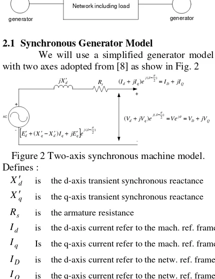
We can describe complex power system as our plant which consists of generators, transmission network as depicted in Fig. 1. It is noted that there can be a number of generators in the system.
Network including load
generator generator
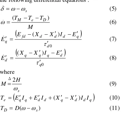
2.1 Synchronous Generator Model
We will use a simplified generator model with two axes adopted from [8] as show in Fig. 2
d
X j ′
s
R
[ ] )
2 (
) (
π δ −
′ + ′ − ′ +
′ j
q q d q
d X X I jEe
E
Q D j q
d jI e I jI
I + ) (−2)= +
(
π δ
Q D j j q
d jV e Ve V jV
V+ − = θ= +
π δ )
2 (
) (
Figure 2 Two-axis synchronous machine model. Defines :
d
X′ is the d-axis transient synchronous reactance
q
X′ is the q-axis transient synchronous reactance
s
R is the armature resistance
d
I is the d-axis current refer to the mach. ref. frame
q
I Is the q-axis current refer to the mach. ref. frame
D
I is the d-axis current refer to the netw. ref. frame
Q
0
q
τ′ is the q-axis transient open circuit time constant
0
d
τ′ is the d-axis transient open circuit time constant
d
X is the d-axis synchronous reactance
q
X is the q-axis synchronous reactance
δ is the angular position of the rotor
ω is the angular velocity of rotor
q
E′ is the q-axis transient voltage
d
E′ is the d-axis transient voltage
fd
E is the DC field voltage
s
ω is the rated value of an angular velocity of rotor
M
T is the mechanical torque applied
e
T is the electromagnetic torque developed
D
T is the damping torque component
D is the damping factor
H is the inertia constant
From the above figure, the stator algebraic equation can be written as :
) 2 (
) )(
(
π δ
θ + + ′ + j −
q d d s j
e jI I X j R Ve
0 ]
) (
[ ′ + ′− ′ + ′ ( 2) =
− −
π δ
j q q d q
d X X I jE e
E
(2)
Multiplying eq. (2) by
) 2 (δ−π
−j
e
and equating the real and the imaginary parts, we obtain :0 )
sin( − − + ′ =
−
′ s d q q
d V R I X I
E δ θ (3)
0 )
cos( − − + ′ =
−
′ s q d d
q V R I X I
E δ θ (4)
In addition, the dynamic behaviors of the rotor motion and the rotor circuits can be describing using the following differential equations :
s
ω ω
δ= − (5)
M T T
TM e D)
( − −
=
ω (6)
(
)
0
) (
d
q d d d fd q
E I X X E E
τ ′
′ − ′ − − = ′
(7)
(
)
0
) (
q
d q q q d
E I X X E
τ′
′ − ′ − = ′
(8)
where
s
H M
ω 2
Δ
= (9)
(
q q d d q d d q)
e E I E I X X I I
T = ′ + ′ +( ′ − ′) (10)
)
( s
D D
T = ω−ω (11)
2.2 Excitation System
In order to improve the damping characteristics of the synchronous generator, supplementary
excitation controls have been widely employed. In this study, we use the IEEE type I exciter as shown in Fig. 3 [8,9].
⎥ ⎦ ⎤ ⎢ ⎣ ⎡
+ F F s sK
τ 1
V ref V
− + −
⎥ ⎦ ⎤ ⎢ ⎣ ⎡
+ A A s K
τ 1
R V +
⎥ ⎦ ⎤ ⎢ ⎣ ⎡
+ E E s
K τ
1
) ( fd EE S
−
fd E
Figure 3 Block diagram of the IEEE type I excitation control.
From the block diagram above, we have three following equations :
E R fd E
fd E E fd
T V E E S K
E = + +
τ
) (
(12)
) (V V K
E K K R K V
V ref
A A fd F A
F A f A
A A
R
R + − + −
− =
τ τ
τ τ
τ
(13)
fdi Fi
Fi F
fi E
K i Rfi R
2
) (τ
τ +
− =
(14)
where
fd E EX B EX
E A e
S = ⋅ × (15)
Defines :
fd
E is the exciter voltage
R
V is the regulator voltage
F
R is the stabilizer voltage
A
K is the voltage regulator gain
A
τ is the voltage regulator time constant
E
K is the exciter gain
E
τ is the exciter time constant
F
K is the regulator stabilizing circuit gain
F
τ is the regulator stabilizing circ time constant
EX
S is the rotating exctr saturation at ceiling voltg
EX
A is the saturation const for rotating exciters
EX
B is the saturation const for rotating exciters
2.3 AC Transmission Network
The network characteristics in this study described in the form of power balance.
The network can consist of many electrical buses and branches depending on the system of interest. Some of the buses connect to the generators and called generator buses. The rest of the buses which are not connected to generating units called as load bus.
The two equations representing real and reactive power balance for each generator bus are given below. For real power balance,
) cos( )
sin( i i qi i i i i
diV I V
I δ −θ + δ −θ
∑
== − − −
n
k
ik k i ik k iV Y
V
1
0 )
cos(θ θ α
(16)
For reactive power balance, ) sin( )
cos( i i qi i i i i
diV I V
I δ −θ + δ −θ
∑
== − −
− n
k
ik k i ik k iV Y
V
1
0 )
sin(θ θ α
(17)
for
i
=
1
,
2
,...,
m
• Load buses
For the load buses, we have equations for both real and reactive power also.
For real power balance,
0 ) cos(
) (
1
= − −
−
∑
=
ik k n
k
i ik k i i
Li V VV Y
P θ θ α (18)
For reactive power balance,
0 ) sin(
) (
1
= − −
−
∑
=
ik k n
k
i ik k i i
Li V VV Y
Q θ θ α (19)
For
i
=
m
+
1
,...
n
Li
P and QLiand are voltage dependence loads. In
this study, loads are assumed as constant power type.
2.4 Initial Condition
It is necessary to compute the initial values of all dynamic states under the given inputs. In power system dynamic analysis, the fixed inputs and initial conditions are normally found from a base case load flow solution, assuming that such load-flow solution exists.
This calculation will be used for linearization process which will be the topic of discussion in the next chapter.
III. LINEARIZED STATE SPACE MODEL OF POWER SYSTEMS
3.1 Linearized State Space Model
The behavior of a dynamic system, such as a power system, may be described by a set of n first order nonlinear ordinary differential equations of the following form :
)
,
(
x
u
f
x
=
(20)
If equations (20) is linearized around the given operating states and inputs (x0,u0), then the linearized state equation can be written as follows :
u B x A x= Δ + Δ
Δ (21)
where
⎥ ⎥ ⎥ ⎥ ⎥
⎦ ⎤
⎢ ⎢ ⎢ ⎢ ⎢
⎣ ⎡
∂ ∂ ∂
∂
∂ ∂ ∂
∂
=
n n n
n
x f x
f
x f x
f A
1
1
1 1
... ... ...
...
⎥ ⎥ ⎥ ⎥ ⎥
⎦ ⎤
⎢ ⎢ ⎢ ⎢ ⎢
⎣ ⎡
∂ ∂ ∂
∂
∂ ∂ ∂
=
r n n
r
u f u
f
u f u
f B
1
1 1
... ... ...
...
(22)
3.2 Eigenvalue and Stability
After the linearized state space representation of the system is obtained such as eq.21, we can see the eigenvalues of the system by inspection of matrix
A
, which reveal the stability of system.A negative real eigenvalue represents a decaying mode. The larger its magnitude, the faster the decay (system stable), while a positive real eigenvalue represent instability
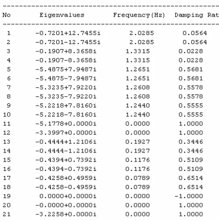
For a complex pair of eigenvalues λ =σ± jω the frequency of oscillation in Hz is given by :
π ω 2
=
f (23)
In addition, the damping ratio can be computed as :
2
2 ω
σ σ ζ
+ −
= (24)
3.3 Participation Factor
Participation factor analysis aids in the identification of how each state variable is reflected on a given mode or eigenvalue. Participation factorpki is defined as
∑
==
n
k ki ik
ik ki ki
w v
w v p
1
(25)
Where
•
p
kiis the participation factor relating theth
k
state variable to thei
theigenvalue•
w
kiandv
kiare thek
th entries in the left and right eigenvector associated with theth
i
eigenvalueA further normalization can be done by making the largest of the participation factors equal to unity.
3.4 Linearized State Space Model of Power Systems
systematic procedure for treating the wide range of devices.
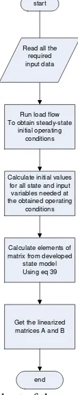
Figure 4 An algorithm to generate linearized state space model.
Fig. 4 shows the steps to get the linearized state space model of power systems. These are those steps :
• Collect differential and algebraic equations a. Generating Unit
1. Four differential equations for generator and three differential equations for exciter : seven differential equations for each generating unit, 7m.
2. Two real stator algebraic equations for each generating unit.
b. Network
1. Two real network equations for each generator bus.
2. Two real network equations for each load bus.
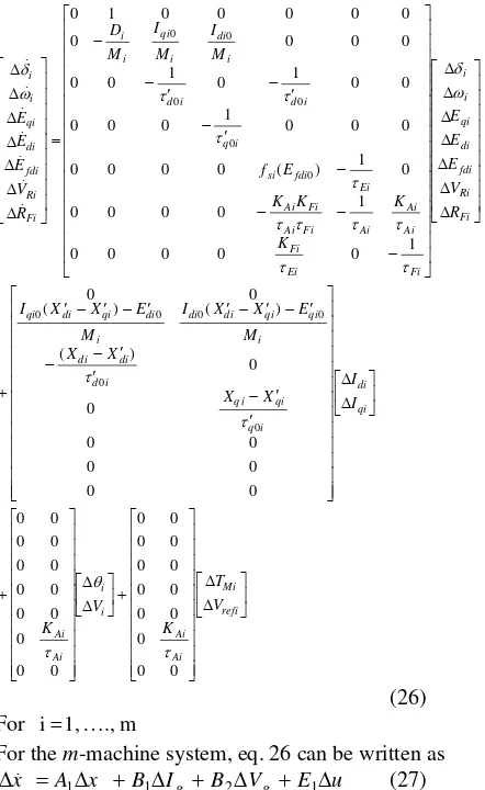
• Linearize all equations with respect to all variables and construct equations in matrix form
1. The linearization of the differential equations from generating unit yields :
⎥
2. Linearized the stator algebraic equations from generating unit yields:
( )
⎥
• Eliminate all variables other than state or input variables
From eq. 27, 29, 31, 33 we need to eliminate
This completes the calculation to get linearized state space model of power systems.
IV. STATE SPACE MODEL GENERATION 4.1 Input Data Preparation
The developed program can handle power system with many numbers of generators and buses. The input which is needed by the program are parameter datas of generators (including exciter) and network. The same network data for load flow studies is used for the calculation.
4.2 Flow Chart of the Program
The first step of the program is read input data from all components. After that the program will run load flow to calculate the operating point of the network. From operating point, program will continue to calculate initial condition all variables in generator. Then program will calculate the matrix for each equation and do many calculations based on the algorithm to develop state model. The flow chart is in Fig. 5 below.
Calculate initial values for all state and input
variables needed at the obtained operating
conditions start
end Run load flow To obtain steady-state
initial operating conditions
Calculate elements of matrix from developed
state model Using eq 39
Get the linearized matrices A and B
Read all the required input data
4.3 Outputs of the Program
The developed program will generate state space representation of the power systems with HVDC link. It produces matrices A and B of the systems. After having these matrices, the program will calculate eigenvalues, frequency of oscillation, damping ratio, participation factor of the system.
The developed program is useful to analyze the small signal stability of the system. We can get the eigenvalues of the system thus we can check the stability of it. We also calculate the frequency of oscillation and damping ratio, thus we can investigate what kind of problem in the system. Moreover, we can see the participation factor to see the participation of states to each mode.
V. TEST RESULTS
The developed program is applied for the Western System Coordinating Council (WSCC) 3-machine, 9-bus system shown in Fig. 6. This system is used to validate the developed program. In literature [8] there are some discussions about this system. They calculate the operating condition from the nominal loading, initial condition of all variables, eigenvalues and participation factor of the system. Those calculation will be compared with the calculation from developed program so that we sure that the developed program is correct.
With the data that we have, we can calculate operating condition of the network by running load flow program. We can see the results in Table 1.
Table 1 Load flow solutions of the WSCC Bus Type of
bus
Voltage Magnitude
(pu)
Voltage Angle (angle)
PG (pu)
QG (pu)
-PL -QL
1 (swing) 1.04 0.000 0.716 0.271 - -
2 (PV) 1.025 9.280 1.63 0.067 - -
3 (PV) 1.025 4.665 0.85
-0.109
- -
4 (PQ) 1.026 -2.217 - - - -
5 (PQ) 0.996 -3.989 - - 1.25 0.5
6 (PQ) 1.013 -3.687 - - 0.9 0.3
7 (PQ) 1.026 3.720 - - - -
8 (PQ) 1.016 0.728 - - 1.00 0.35
9 (PQ) 1.032 1.967 - - - -
After we get operating point from running load flow program, we will calculate initial variables in the system. The computed initial conditions are given in Table 2.
Table 2. Computed initial conditions Variables Gen 1 Gen 2 Gen 3
δ 3.5860 61.0980 54.1370
d
I 0.303 1.290 0.561
q
I 0.671 0.932 0.619
d
V 0.065 0.806 0.779
q
V 1.038 0.634 0.666
d
E′ 0 0.622 0.624
d
E′ 1.056 0.788 0.768
fd
E 1.082 1.789 1.403
f
R 0.195 0.322 0.253
R
V 1.105 1.902 1.451
ref
V 1.095 1.120 1.098
M
T 0.716 1.630 0.850
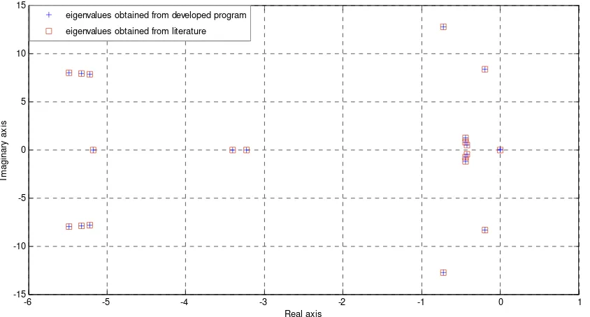
In this system we have three generators and each generator has 7 states. Its mean, we will have 21 states. After we get operating point of network and initial condition of all variables, we can compute the matrices A and B. After that the program will give eigenvalues, frequency and damping ratio of the system (see Table 3). Fig. 7 lists the comparison of eigenvalues obtained from developed program and literature [8] for the WSCC system.
Figure 6 A single line diagram of the Western System Coordinating Council (WSCC)
-6 -5 -4 -3 -2 -1 0 1
-15 -10 -5 0 5 10 15
Real axis
Im
agi
nar
y
ax
is
eigenvalues obtained from developed program eigenvalues obtained from literature [14]
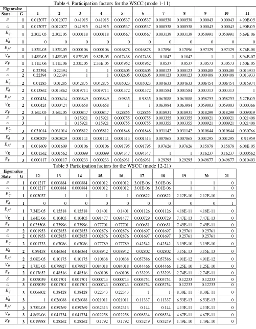
For the participation factor, we get :
Table 4. Participation factors for the WSCC (mode 1-11) Eigenvalue
State G 1 2 3 4 5 6 7 8 9 10 11
δ 1 0.012077 0.012077 0.41915 0.41915 0.000537 0.000537 0.000538 0.000538 0.00043 0.00043 4.90E-05
ω 1 0.012077 0.012077 0.41915 0.41915 0.000537 0.000537 0.000538 0.000538 0.00043 0.00043 4.90E-05
q
E′ 1 2.30E-05 2.30E-05 0.000118 0.000118 0.000567 0.000567 0.003139 0.003139 0.050991 0.050991 5.69E-06
d
E′ 1 0 0 0 0 0 0 0 0 0 0 0
fd
E 1 1.52E-05 1.52E-05 0.000106 0.000106 0.016878 0.016878 0.17896 0.17896 0.97329 0.97329 8.76E-08
R
V 1 1.48E-05 1.48E-05 9.82E-05 9.82E-05 0.017438 0.017438 0.1842 0.1842 1 1 8.94E-07
F
R 1 1.11E-06 1.11E-06 2.33E-05 2.33E-05 0.004952 0.004952 0.0537 0.0537 0.30573 0.30573 1.50E-05
δ 2 0.22394 0.22394 1 1 0.002605 0.002605 0.000123 0.000123 0.000408 0.000408 0.013933
ω 2 0.22394 0.22394 1 1 0.002605 0.002605 0.000123 0.000123 0.000408 0.000408 0.013933
q
E′ 2 0.01285 0.01285 0.042875 0.042875 0.035023 0.035023 0.004633 0.004633 0.006454 0.006454 0.015974
d
E′ 2 0.013862 0.013862 0.019714 0.019714 0.004372 0.004372 0.001584 0.001584 0.003313 0.003313 1
fd
E 2 0.000434 0.000434 0.003849 0.003849 0.9835 0.9835 0.063088 0.063088 0.058253 0.058253 5.27E-05
R
V 2 0.000424 0.000424 0.003658 0.003658 1 1 0.063984 0.063984 0.059003 0.059003 0.000366
F
R 2 3.16E-05 3.16E-05 0.000847 0.000847 0.28855 0.28855 0.018931 0.018931 0.018299 0.018299 0.009019
δ 3 1 1 0.15921 0.15921 0.000755 0.000755 0.003355 0.003355 0.000921 0.000921 0.021408
ω 3 1 1 0.15921 0.15921 0.000755 0.000755 0.003355 0.003355 0.000921 0.000921 0.021408
q
E′
3 0.031014 0.031014 0.005812 0.005812 0.001848 0.001848 0.031142 0.031142 0.010844 0.010844 0.030766
d
E′ 3 0.080829 0.080829 0.001141 0.001141 0.001313 0.001313 0.007865 0.007865 0.001295 0.001295 0.91959
fd
E
3 0.001609 0.001609 0.00106 0.00106 0.091795 0.091795 0.97626 0.97626 0.15878 0.15878 6.08E-05
R
V 3 0.001562 0.001562 0.00099 0.00099 0.094347 0.094347 1 1 0.16237 0.16237 0.000562
F
R 3 0.000117 0.000117 0.000233 0.000233 0.026931 0.026931 0.29295 0.29295 0.049877 0.049877 0.010403
Table 5 Participation factors for the WSCC (mode 12-21) Eigenvalue
State G 12 13 14 15 16 17 18 19 20 21
δ 1 0.001217 0.000884 0.000884 0.001012 0.001012 3.01E-06 3.01E-06 1 1 0
ω 1 0.001217 0.000884 0.000884 0.001012 0.001012 3.01E-06 3.01E-06 1 1 0
q
E′
1 0.003037 1 1 1 1 0.00822 0.00822 2.12E-10 2.12E-10 0
d
E′ 1 0 0 0 0 0 0 0 0 0 1
fd
E
1 7.34E-05 0.15518 0.15518 0.1401 0.1401 0.001126 0.001126 4.18E-11 4.18E-11 0
R
V 1 1.64E-06 0.10405 0.10405 0.091477 0.091477 0.000729 0.000729 7.47E-13 7.47E-13 0
F
R 1 0.025508 0.73996 0.73996 0.77701 0.77701 0.00651 0.00651 7.45E-11 7.45E-11 0
δ 2 0.001953 0.002853 0.002853 0.002876 0.002876 0.001697 0.001697 0.25761 0.25761 0
ω 2 0.001953 0.002853 0.002853 0.002876 0.002876 0.001697 0.001697 0.25761 0.25761 0
q
E′
2 0.001733 0.67086 0.67086 0.77789 0.77789 0.42542 0.42542 3.19E-10 3.19E-10 0
d
E′ 2 0.89458 0.046364 0.046364 0.038942 0.038942 0.02802 0.02802 3.15E-13 3.15E-13 0
fd
E 2 5.08E-05 0.10175 0.10175 0.10838 0.10838 0.057586 0.057586 4.91E-12 4.91E-12 0
R
V 2 1.73E-05 0.079927 0.079927 0.084018 0.084018 0.044466 0.044466 1.25E-10 1.25E-10 0
F
R 2 0.017652 0.48516 0.48516 0.60108 0.60108 0.33293 0.33293 2.74E-11 2.74E-11 0
δ 3 0.009039 0.001701 0.001701 0.000743 0.000743 0.003754 0.003754 0.12233 0.12233 0
ω 3 0.009039 0.001701 0.001701 0.000743 0.000743 0.003754 0.003754 0.12233 0.12233 0
q
E′
3 0.006602 0.38428 0.38428 0.22343 0.22343 1 1 8.30E-11 8.30E-11 0
d
E′ 3 1 0.026088 0.026088 0.021011 0.021011 0.11337 0.11337 6.53E-13 6.53E-13 0
fd
E
3 5.75E-05 0.059269 0.059269 0.032313 0.032313 0.144 0.144 4.13E-11 4.13E-11 0
R
V 3 4.86E-06 0.041734 0.041734 0.022258 0.022258 0.098534 0.098534 4.67E-11 4.67E-11 0
F
VI.CONCLUSION
The developed program can handle calculating state space representation of actual power systems which consist of generating units and network.
Eigenvalues, frequency, damping ratio and participation factor can be computed.
From the result we see that the obtained eigenvalues and participation factor of WSCC are correct.
VII. REFERENCES
1. K.R. Padiyar, M.A. Pai, C.
Radhakrishna, “A versatile system model for the dynamic stability analysis of power systems including HVDC links”, IEEE Transaction on Power System, 1981, P: 1871-1879.
2. Prabha Kundur, Power System Stability and Control. New York: McGraw-Hill, Inc, 1994.
3. P.K. Dash, A. Liew , A. Routray, “Design of robust controllers for HVDC links in AC-DC power system”, Electric Power System Research, 1995, P: 201-209.
4. K.G. Narendra, K. Khorasani, V.K. Sood, R. V. Patel, “Intelligent current controller for an HVDC transmission link”, IEEE Transacntion on Power Systems, voltage 13, no 3, August (1998) : 1076:1083.
5. Katsuhiko Ogata, Modern Control
Engineering, Prentice Hall
International, Inc, 1997.
6. A.S. AlFuhaid, M.S. Mahmoud, M.A. El-Sayed, “Modelling and control of high-voltage AC- DC power systems”, Journal of the Franklin Institut”, 1999, P: 767- 781.
7. V.Vittal, M.H. Khammash, C.D.
Pawloski, “Analysis of control performance for stability robustness of power system“, Proceeding of the 32nd Conference on Decision and Control, San Antonio, Texas, 1993.
8. Peter W. Sauer, M.A. PAI, Power System Dynamics and Stability, Prentice Hall, 1998.
9. P.M. Anderson, A.A Fouad, Power System Control and Stability, The Iowa State University Press, 1997
10. Katsuhiko Ogata, State Space Analysis of Control Systems, Prentice Hall International, Inc, 1967
11. William L. Brogan, Modern Control Theory, Prentice Hall International Edition, 1991.